Fundamentals of Inference

Overview

Bedrock for everything else: probability spaces, conditioning, and information measures. Later chapters reuse these definitions verbatim.

Figure 1: Conditioning an event \(A\) on another event \(B\) can be understood as replacing the universe of all possible outcomes \(\Omega\) by the observed outcomes \(B\). Then, the conditional probability is simply expressing the likelihood of \(A\) given that \(B\) occurred.

Probability spaces and viewpoints

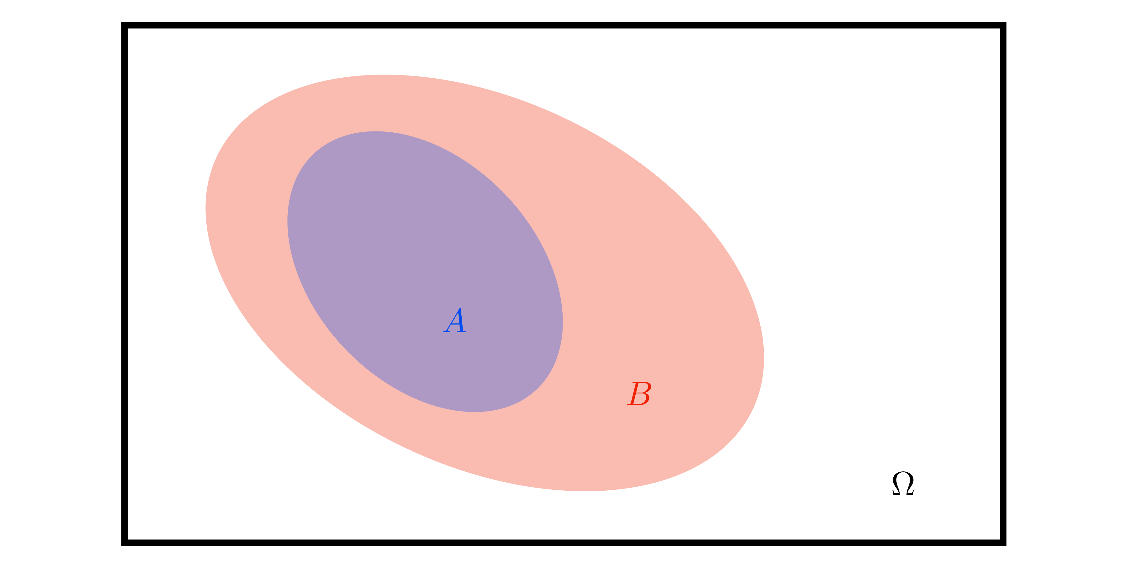
Probability space \((\Omega,\mathcal{A},\mathbb{P})\): outcome space, \(\sigma\)-algebra, and measure with \(\mathbb{P}(\Omega)=1\); Borel \(\sigma\)-algebra for \(\mathbb{R}^d\).
Frequentist view: \(\Pr[A]=\lim_{N\to\infty}\frac{1}{N}\sum_{i=1}^N\mathbf{1}\{A\text{ occurs in trial }i\}\) when IID replicates exist.
Bayesian view: \(\Pr[A]\) encodes coherent belief; Dutch-book coherence ⇒ Kolmogorov axioms. Prior/posterior updates by Bayes’ rule.

Random variables and transformations

Measurable map \(X:(\Omega,\mathcal{A})\to(\mathcal{X},\mathcal{B})\) pushes forward \(\mathbb{P}\) to \(P_X\).
Discrete: PMF \(p_X(x)=\Pr[X=x]\), CDF \(F_X(x)=\Pr[X\le x]\).
Continuous: PDF \(p_X\) with \(\Pr[X\in S]=\int_S p_X(x)\,dx\).
Support \(\text{supp}(p)=\{x:p(x)>0\}\) is crucial for conditioning (e.g., KL terms later).
Change of variables: for invertible \(g\) with Jacobian \(J\), \(p_Y(y)=p_X(g^{-1}(y))\left|\det J_{g^{-1}}(y)\right|\).

Conditioning identities

Product rule: \(\Pr[A,B]=\Pr[A\mid B]\Pr[B]\).
Law of total probability: \(\Pr[A]=\sum_i\Pr[A\mid B_i]\Pr[B_i]\) or \(\int \Pr[A\mid b]p_B(b)db\).
Bayes’ rule: \(\Pr[B\mid A]=\frac{\Pr[A\mid B]\Pr[B]}{\Pr[A]}\); density form \(p_{X\mid Y}(x\mid y)=p_{X,Y}(x,y)/p_Y(y)\).
Tower property: \(\mathbb{E}[X]=\mathbb{E}_Y[\mathbb{E}[X\mid Y]]\); used repeatedly in variance decompositions and TD learning.

Expectations, variance, covariance

Expectation linear; Jensen: convex \(g\) ⇒ \(g(\mathbb{E}[X])\le\mathbb{E}[g(X)]\) (applied in KL bounds, ELBO derivations).
Variance: \(\operatorname{Var}[X]=\mathbb{E}[X^2]-\mathbb{E}[X]^2\); covariance matrix \(\Sigma_X=\mathbb{E}[(X-\mathbb{E}X)(X-\mathbb{E}X)^\top]\) PSD.
Linear maps: \(\operatorname{Var}[AX+b]=A\operatorname{Var}[X]A^\top\); Schur complement yields conditional covariance (used in GP conditioning, Kalman filters).
Law of total variance: \(\operatorname{Var}[X]=\mathbb{E}_Y[\operatorname{Var}[X\mid Y]]+\operatorname{Var}_Y(\mathbb{E}[X\mid Y])\) ⇒ interprets aleatoric vs epistemic uncertainty.

Independence notions

\(X\perp Y\) iff joint factorizes; conditional independence \(X\perp Y\mid Z\) iff \(p(x,y\mid z)=p(x\mid z)p(y\mid z)\).
Pairwise independence ≠ mutual independence; counterexamples show up in mixture models.
Gaussian special case: zero covariance ⇔ independence.

Multivariate Gaussian essentials

PDF: \(\mathcal{N}(x\mid\mu,\Sigma)\) with determinant and quadratic form.
Affine invariance: \(AX+b\sim\mathcal{N}(A\mu+b, A\Sigma A^\top)\).
Sampling: \(x=\mu+L\xi\), \(\xi\sim\mathcal{N}(0,I)\) (Cholesky or spectral) — reused for GP sampling, latent variable models.
Conditioning on block partitions: \[X_A\mid X_B=b \sim \mathcal{N}(\mu_A + \Sigma_{AB}\Sigma_{BB}^{-1}(b-\mu_B),\; \Sigma_{AA}-\Sigma_{AB}\Sigma_{BB}^{-1}\Sigma_{BA}).\] Schur complement PSD ⇒ conditioning never increases variance (core to GP posterior, Kalman updates).

Parameter estimation summary

Likelihood \(p(\mathcal{D}\mid\theta)=\prod_i p(y_i\mid x_i,\theta)\); MLE solves \(\max_\theta \ell(\theta)=\sum_i \log p(y_i\mid x_i,\theta)\).
MAP adds prior \(\log p(\theta)\); recovers ridge/lasso when using quadratic penalties.
Bayesian predictive: \(p(y^*\mid x^*,\mathcal{D})=\int p(y^*\mid x^*,\theta)p(\theta\mid\mathcal{D})d\theta\); motivates maintaining posterior rather than point estimates.

Information-theoretic quantities

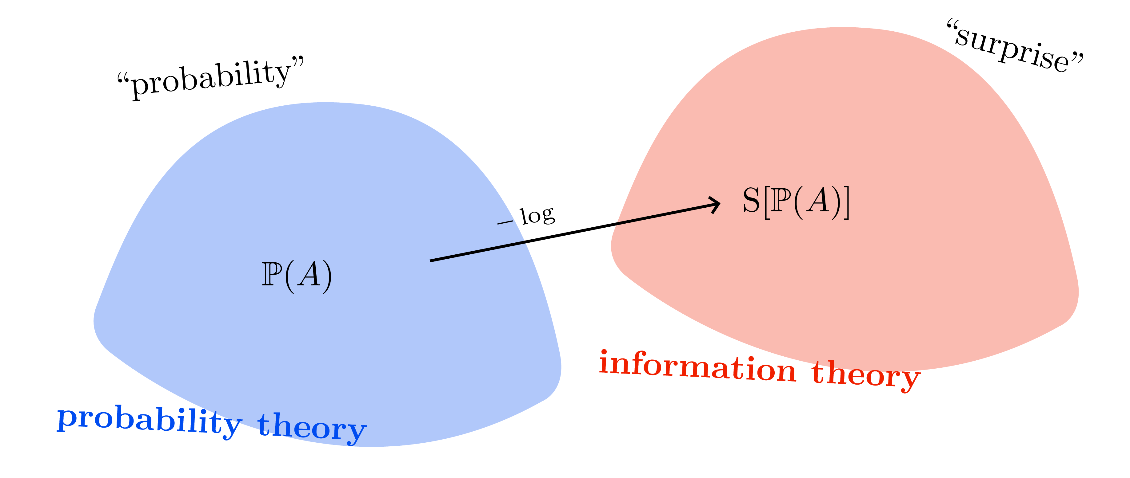
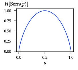
Figure 2: Probability space (left) and the corresponding surprise space obtained via the \(-\log\) transform.

Figure 3: Entropy of a Bernoulli experiment as a function of the success probability \(p\).

Surprise \(\mathcal{S}(u)=-\log u\); entropy \(H(p)=\mathbb{E}_p[-\log p(X)]\) measures average surprise.
Cross-entropy \(H(p,q)=\mathbb{E}_p[-\log q(X)]\).
KL divergence \(\mathrm{KL}(p\|q)=\mathbb{E}_p\big[\log\frac{p}{q}\big]\ge0\); forward KL is mode-covering, reverse KL is mode-seeking.
Mutual information \(I(X;Y)=H(X)-H(X\mid Y)\) underlies active learning, Bayesian optimization, and exploration bonuses.

Keep this sheet handy: every later derivation (Bayesian linear regression, VI, Kalman filtering, GP conditioning, RL entropy bonuses) is a remix of these identities.

Bayesian Linear Regression

Overview

First Bayesian workhorse: converts linear regression into a full posterior. Sets up the probabilistic tools reused by later chapters.

Figure 4: Bayesian linear regression written as a plate diagram.

Linear-Gaussian model recap

Data: inputs \(\mathbf{X}\in\mathbb{R}^{n\times d}\), labels \(\mathbf{y}\in\mathbb{R}^n\).
Likelihood \(p(\mathbf{y}\mid\mathbf{w})=\prod_{i=1}^n \mathcal{N}(y_i\mid\mathbf{x}_i^\top\mathbf{w},\sigma_n^2)\) — Gaussian noise \(\varepsilon_i\sim\mathcal{N}(0,\sigma_n^2)\).
Prior \(\mathbf{w}\sim\mathcal{N}(0,\sigma_p^2 I)\) ⇒ conjugate; ridge/MAP arises when replacing posterior with its mode.

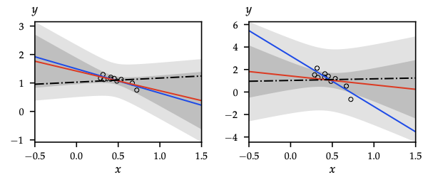
Figure 5: Comparison of least-squares, ridge regression, and Bayesian linear regression fits together with posterior uncertainty bands.

Posterior (complete the square): \[ \Sigma = (\sigma_n^{-2}\mathbf{X}^\top\mathbf{X} + \sigma_p^{-2}I)^{-1},\quad \mu = \sigma_n^{-2}\Sigma\mathbf{X}^\top\mathbf{y},\quad p(\mathbf{w}\mid\mathcal{D})=\mathcal{N}(\mu,\Sigma). \]
Posterior collapses to MLE as \(\sigma_p^2\to\infty\); to prior as \(n\to0\).

Predictive distribution & variance decomposition

Latent function \(f^* = \mathbf{x}_*^\top\mathbf{w}\) yields \(f^*\mid\mathcal{D},\mathbf{x}_*\sim\mathcal{N}(\mathbf{x}_*^\top\mu,\mathbf{x}_*^\top\Sigma\mathbf{x}_*)\).
Observed target \(y^*\mid\mathcal{D},\mathbf{x}_*\sim\mathcal{N}(\mathbf{x}_*^\top\mu,\mathbf{x}_*^\top\Sigma\mathbf{x}_* + \sigma_n^2)\).
Using law of total variance, predictive variance splits into epistemic \(\mathbf{x}_*^\top\Sigma\mathbf{x}_*\) (shrinks with data) + aleatoric \(\sigma_n^2\) (irreducible noise).

Online / Kalman-style updates

Start with \((\mu^{(0)},\Sigma^{(0)})=(0,\sigma_p^2 I)\).
Assimilate \((\mathbf{x}_t,y_t)\) via gain \(k_t = \frac{\Sigma^{(t-1)}\mathbf{x}_t}{\sigma_n^2+\mathbf{x}_t^\top\Sigma^{(t-1)}\mathbf{x}_t}\): \[ \mu^{(t)} = \mu^{(t-1)} + k_t(y_t - \mathbf{x}_t^\top\mu^{(t-1)}),\quad \Sigma^{(t)} = \Sigma^{(t-1)} - k_t\mathbf{x}_t^\top\Sigma^{(t-1)}. \]
Identical algebra to Kalman filtering with a static state; cost \(\mathcal{O}(d^2)\) per update.

Function-space view and kernels

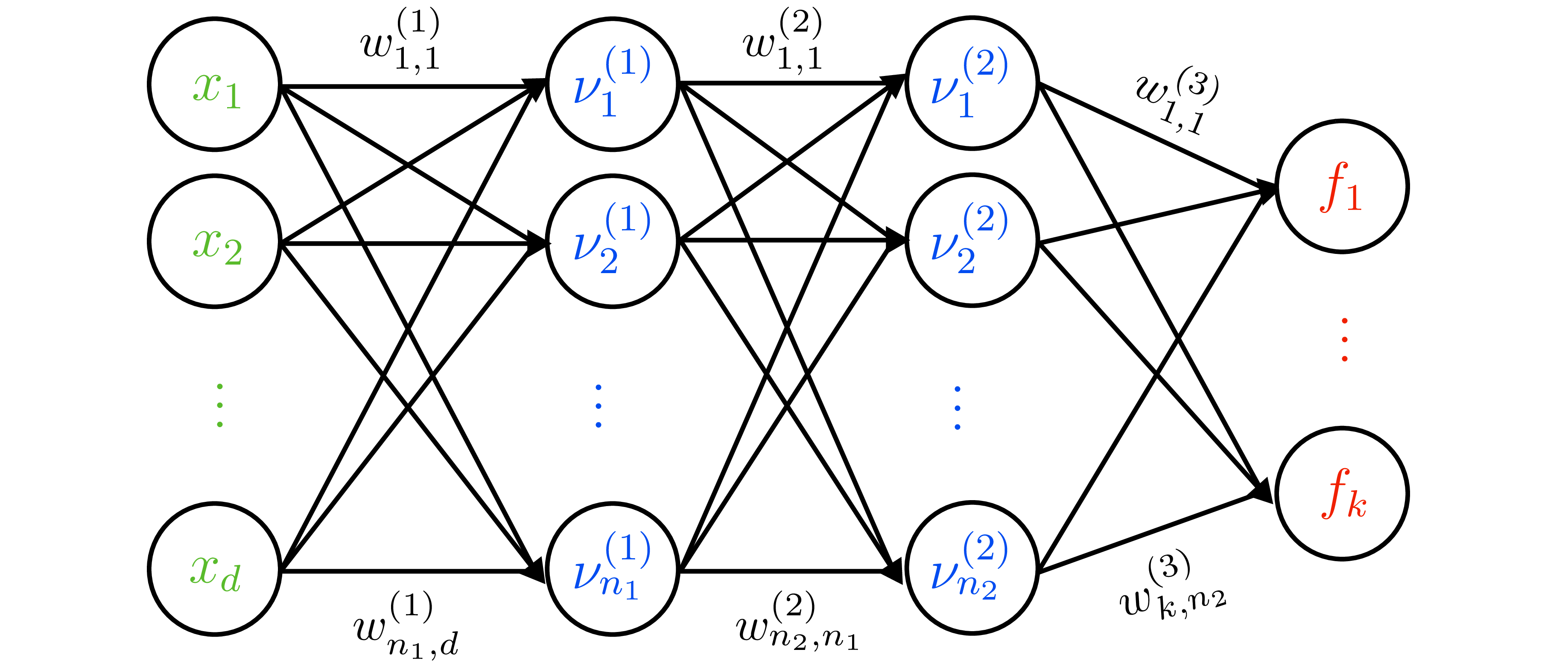
Figure 6: Computation graph of a feed-forward neural network with two hidden layers.

Transform features with \(\boldsymbol{\phi}(x)\) (possibly infinite). Weight prior induces function prior: \[ f\mid\mathbf{X} \sim \mathcal{N}(0,\mathbf{K}),\quad K_{ij}=\sigma_p^2\,\boldsymbol{\phi}(\mathbf{x}_i)^\top\boldsymbol{\phi}(\mathbf{x}_j) = k(\mathbf{x}_i,\mathbf{x}_j). \]
Predictive mean \(\mu'(x)=k(x,\mathbf{X})^{\top}(\mathbf{K}+\sigma_n^2 I)^{-1}\mathbf{y}\), predictive variance \(k'(x,x)=k(x,x)-k(x,\mathbf{X})^{\top}(\mathbf{K}+\sigma_n^2 I)^{-1}k(x,\mathbf{X})\).
Removes need to explicitly materialize high-dimensional \(\boldsymbol{\phi}\) — the kernel trick in action.

Evidence maximization / empirical Bayes

Marginal likelihood (evidence) of labels: \[ \log p(\mathbf{y}\mid\mathbf{X},\theta) = -\tfrac{1}{2}\mathbf{y}^\top\mathcal{C}^{-1}\mathbf{y} - \tfrac{1}{2}\log|\mathcal{C}| - \tfrac{n}{2}\log 2\pi, \] where \(\mathcal{C}=\sigma_n^2 I + \sigma_p^2 \mathbf{X}\mathbf{X}^\top\) and \(\theta=(\sigma_n,\sigma_p)\).
Maximizing evidence trades fit term \(\mathbf{y}^\top\mathcal{C}^{-1}\mathbf{y}\) vs complexity term \(\log|\mathcal{C}|\); useful for hyperparameter tuning across Bayesian models.

Design choices & links forward

Regularization perspective: prior variance \(\sigma_p^2\) controls weight shrinkage (ridge); different priors (Laplace, hierarchical) lead to sparse or hierarchical BLR.
Posterior covariance \(\Sigma\) is the raw material for Thompson sampling, Bayesian optimization, and epistemic bonuses in model-based RL.
Function-space formulation + evidence maximization form the blueprint for Gaussian processes, variational inference, and dropout-as-variational inference.

Bayesian Filtering

Overview

Sequential inference over hidden states. Kalman filtering is the linear-Gaussian case; smoothing/prediction variants reappear in downstream planning settings.

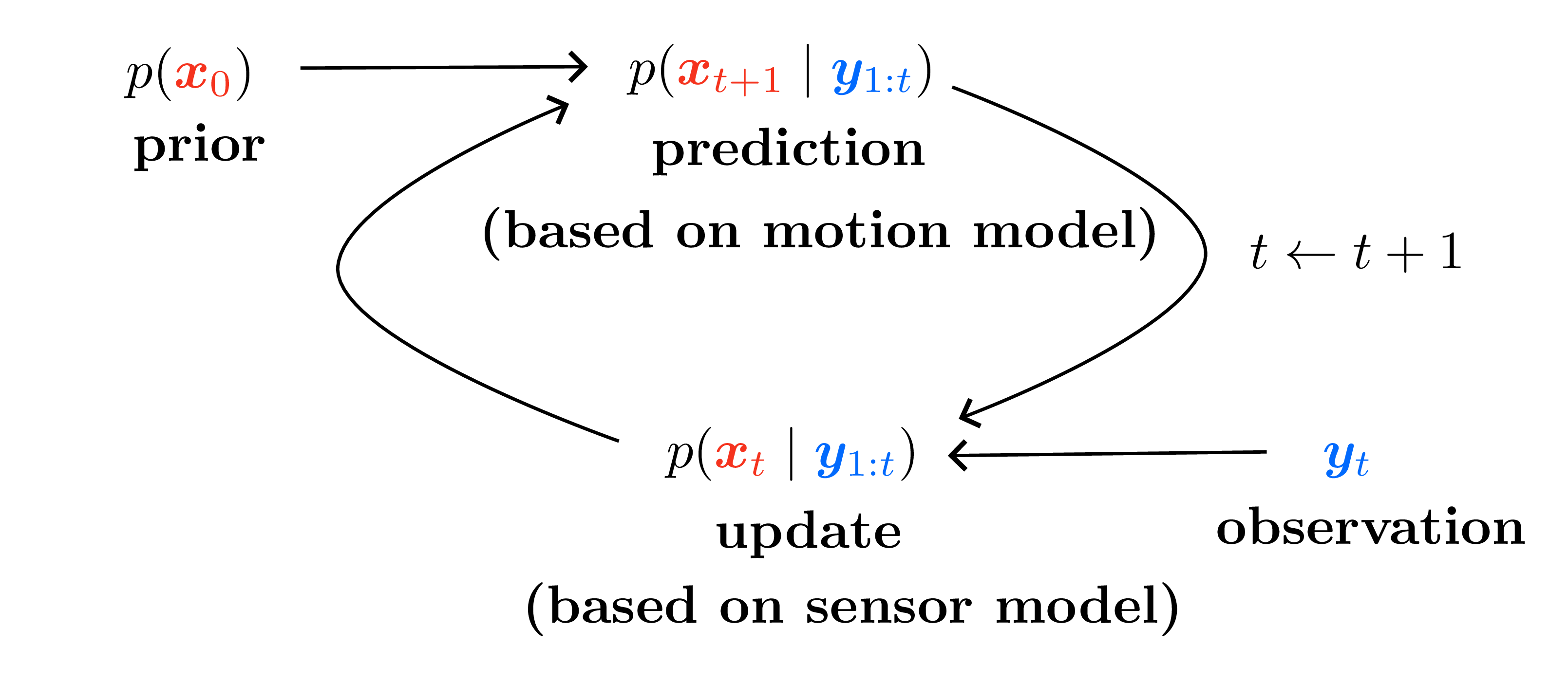
Figure 7: Bayesian filtering: perceive the world state and update the latent belief.

Linear-Gaussian state-space model

Latent state \(x_t\in\mathbb{R}^d\), observation \(y_t\in\mathbb{R}^m\).
Dynamics (motion) \(x_{t+1}=Fx_t+\varepsilon_t\), \(\varepsilon_t\sim\mathcal{N}(0,\Sigma_x)\).
Observation (sensor) \(y_t=Hx_t+\eta_t\), \(\eta_t\sim\mathcal{N}(0,\Sigma_y)\).
Prior \(x_0\sim\mathcal{N}(\mu_0,\Sigma_0)\); noises independent.
Graphical model (Figure 8): Markov property \(x_{t+1}\perp x_{0:t-1},y_{0:t-1}\mid x_t\); measurement independence \(y_t\perp x_{0:t-1},y_{0:t-1}\mid x_t\).

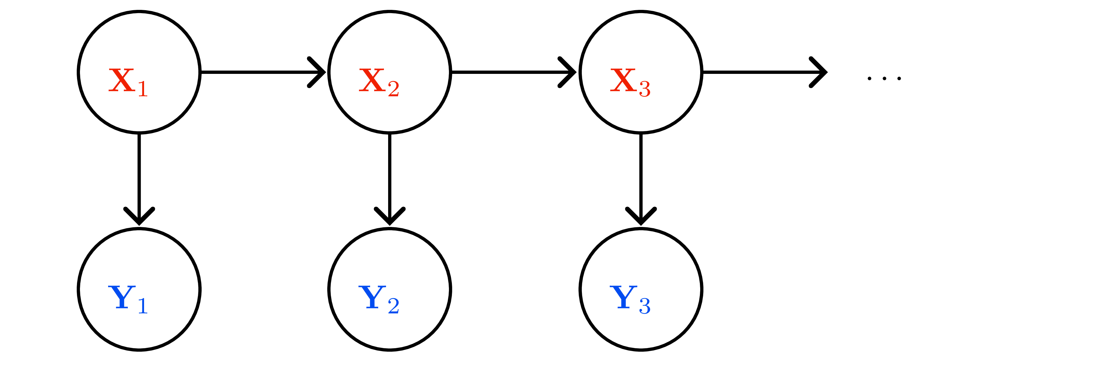
Figure 8: Graphical model of a Kalman filter with hidden states \(X_t\) and observations \(Y_t\).

Kalman filter recursion

Belief \(p(x_t\mid y_{1:t}) = \mathcal{N}(\mu_t,\Sigma_t)\).

Predict (time update) \[\hat{\mu}_{t+1}=F\mu_t,\qquad \hat{\Sigma}_{t+1}=F\Sigma_t F^\top + \Sigma_x.\]
Update (measurement)
- Kalman gain \(K_{t+1}=\hat{\Sigma}_{t+1}H^\top(H\hat{\Sigma}_{t+1}H^\top+\Sigma_y)^{-1}\).
- Posterior mean/covariance: \[ \mu_{t+1}=\hat{\mu}_{t+1}+K_{t+1}(y_{t+1}-H\hat{\mu}_{t+1}),\quad \Sigma_{t+1}=(I-K_{t+1}H)\hat{\Sigma}_{t+1}. \]

Innovation \(y_{t+1}-H\hat{\mu}_{t+1}\) measures sensor surprise; \(K_{t+1}\) balances trust between prediction and measurement.

Scalar intuition

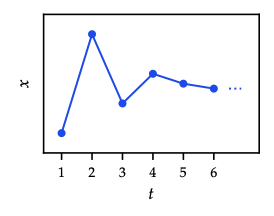
Random walk + noisy sensor: \(x_{t+1}=x_t+\varepsilon_t\), \(y_{t+1}=x_{t+1}+\eta_{t+1}\) with variances \(\sigma_x^2,\sigma_y^2\).
Posterior variance update \(\sigma_{t+1}^2=(1-\lambda)(\sigma_t^2+\sigma_x^2)\) where \[\lambda=\frac{\sigma_t^2+\sigma_x^2}{\sigma_t^2+\sigma_x^2+\sigma_y^2}.\]
\(\sigma_y^2\to0\) ⇒ trust measurements; \(\sigma_y^2\to\infty\) ⇒ ignore measurements.

Figure 9: Hidden states tracked during a one-dimensional random walk example.

Smoothing, prediction, control

Prediction: output \(\mathcal{N}(\hat{\mu}_{t+1},\hat{\Sigma}_{t+1})\) (no measurement).
Filtering: recursion above.
Smoothing: backward pass (Rauch–Tung–Striebel) refines past states once future measurements available — key in EM for LDS.
These three modes generalize to nonlinear filters (EKF/UKF) and particle filters when Gaussian assumptions fail.

Link to Bayesian linear regression

Treat weights \(w\) as static hidden state: \(F=I\), \(\Sigma_x=0\), \(H_t=\mathbf{x}_t^\top\), measurement \(y_t\) ⇒ Kalman filter updates reduce to sequential Bayesian linear regression.
Kalman gain matches recursive least squares gain.

Practical remarks

Time-invariant \((F,H,\Sigma_x,\Sigma_y)\) ⇒ \(K_t\) converges; can precompute steady-state solution via Riccati equation.
Initialization: choose \((\mu_0,\Sigma_0)\) to encode prior belief; large \(\Sigma_0\) yields “cold start” with aggressive measurement uptake.
Failure modes: unmodeled dynamics, non-Gaussian noise ⇒ need EKF/UKF, particle filters, or learned process models.

This chapter’s algebra (matrix Riccati, innovation form) underpins belief updates in POMDPs and latent world models alike.

Gaussian Processes

Overview

Infinite-dimensional generalization of Bayesian linear regression. Kernels encode function priors; posterior algebra mirrors BLR but now happens in function space.

Figure 10: Bayesian optimization loop: observe \(y_t = f(x_t) + \varepsilon_t\) after querying \(x_t\).

Definition

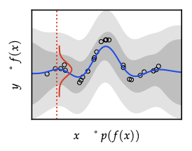
A Gaussian process \(f\sim\mathcal{GP}(\mu,k)\) assigns to every finite index set \(\mathcal{A}=\{x_1,\dots,x_m\}\) a joint Gaussian \(\mathbf{f}_{\mathcal{A}}\sim\mathcal{N}(\mu_{\mathcal{A}},K_{\mathcal{A}\mathcal{A}})\) with \((K_{\mathcal{A}\mathcal{A}})_{ij}=k(x_i,x_j)\).
Observation model: \(y_i=f(x_i)+\varepsilon_i\), \(\varepsilon_i\sim\mathcal{N}(0,\sigma_n^2)\) independent.
Prior predictive at \(x\): \(y\mid x\sim\mathcal{N}(\mu(x), k(x,x)+\sigma_n^2)\).

Figure 11: Gaussian processes behave like infinite-dimensional Gaussians: blue mean function with dark (epistemic) and light (aleatoric) uncertainty bands.

Posterior conditioning (same algebra as BLR)

Given training data \((\mathbf{X},\mathbf{y})\), define \(K=K_{\mathbf{X}\mathbf{X}}\) and \(k_x = k(x,\mathbf{X})\). Posterior is \[ f\mid\mathcal{D} \sim \mathcal{GP}(\mu',k'), \] with \[ \mu'(x)=\mu(x)+k_x^{\top}(K+\sigma_n^2 I)^{-1}(\mathbf{y}-\mu_{\mathbf{X}}), \] \[ k'(x,x')=k(x,x')-k_x^{\top}(K+\sigma_n^2 I)^{-1}k_{x'}. \] Predictive label variance adds \(\sigma_n^2\) back in. Conditioning always reduces covariance (Schur complement PSD).

Sampling

Direct: draw \(\xi\sim\mathcal{N}(0,I)\) and compute \(f=\mu + L\xi\) with \(L\) Cholesky of \(K\) (\(\mathcal{O}(n^3)\)).
Forward sampling: generate points sequentially using conditional Gaussians (same complexity but conceptually useful for illustration).

Kernels

Valid kernel iff Gram matrix PSD for any finite set; closure under sum/product/positive scaling/polynomials/\(\exp\).
Stationary \(k(x,x')=\tilde{k}(x-x')\); isotropic depends only on \(\|x-x'\|\).
Important families:
- Linear \(k(x,x')=\sigma_p^2 x^\top x'\) ↔︎ BLR.
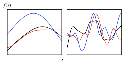
- Squared exponential (RBF) \(\exp(-\|x-x'\|^2/(2\ell^2))\) → infinitely smooth.
- Matérn \((\nu,\ell)\) controls differentiability (# of mean-square derivatives \(=\lfloor\nu\rfloor\)); Laplace is Matérn \(\nu=1/2\).
- Periodic, rational quadratic, ARD kernels for anisotropy.

Figure 12: Functions sampled from an RBF kernel GP with length scales \(h=5\) (left) and \(h=1\) (right).

Feature-space story: \(k(x,x')=\phi(x)^\top\phi(x')\) (Mercer). Random Fourier features approximate stationary kernels via Bochner.

Hyperparameter selection

Marginal likelihood \(p(\mathbf{y}\mid\mathbf{X},\theta)=\mathcal{N}(0,K_{\theta}+\sigma_n^2 I)\).
Log-evidence (Eq. 4.18) balances data fit \(\mathbf{y}^\top K^{-1}\mathbf{y}\) vs complexity \(\log|K|\).
Optimize wrt kernel parameters (\(\ell\), signal variance, noise) via gradient-based methods; derivatives involve trace identities.
Bayesian treatment: put priors on hyperparameters and integrate (costly; approximations via HMC/VI possible).

Scalability / approximations

Exact cost \(\mathcal{O}(n^3)\) ⇒ approximations needed for large \(n\).
Local/sparse methods: inducing points (FITC, VFE), Nyström approximations, structured kernel interpolation.
Feature approximations: random Fourier features (stationary kernels), orthogonal random features, sketching.
Kron/Toeplitz exploitation for grid inputs.

Connections forward

GP posterior mean = kernel ridge regression estimate; posterior variance drives exploration bonuses and safety analysis.
Evidence maximization parallels empirical Bayes in BLR and hyperparameter tuning in Bayesian neural nets.
Kernels express prior assumptions; in Bayesian optimization they define smoothness and drive acquisition functions.

Variational Inference

Overview

Approximate Bayesian inference by optimization. Provides the ELBO machinery that powers probabilistic deep learning, RL, and latent world models.

Figure 13: An illustration of variational inference in the space of distributions \(\spP\). The variational distribution \(\qs \in \spQ\) is the optimal approximation of the true posterior \(p\).

From Laplace to VI

Laplace: second-order Taylor of log-posterior around MAP \(\hat{\theta}\) ⇒ Gaussian \(q(\theta)=\mathcal{N}(\hat{\theta},(-\nabla^2\log p)^{-1})\). Good for unimodal, local approximations; ignores skew/tails.

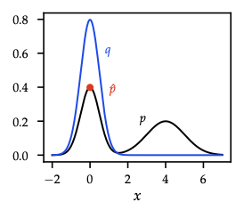
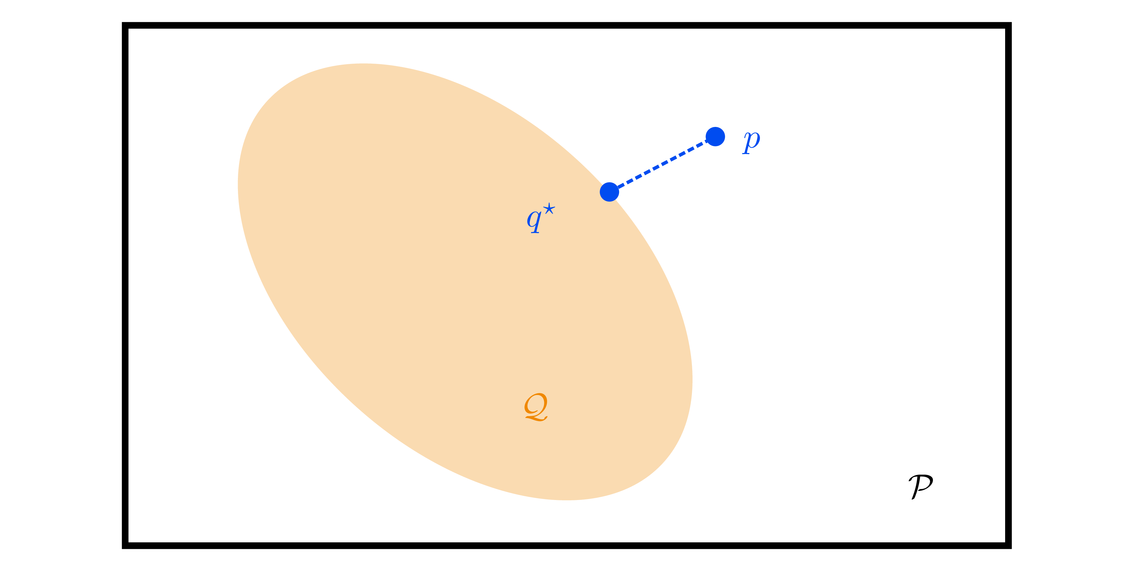
Figure 14: Laplace approximation \(q\) around the mode of \(p\); it matches local curvature but can be overly confident away from the mode.

Variational inference generalizes: choose family \(\mathcal{Q}=\{q_{\lambda}(\theta)\}\), solve \[q^* = \arg\min_{q\in\mathcal{Q}} \mathrm{KL}(q\|p(\theta\mid\mathcal{D})).\] Reverse KL is mode-seeking (prefers concentrated approximations), complementing forward-KL moment-matching (EM-style) in exponential families.

ELBO identities

Evidence lower bound (ELBO): \[\mathcal{L}(q)=\mathbb{E}_q[\log p(\mathcal{D},\theta)] + \mathcal{H}(q).\]
Relationship: \(\log p(\mathcal{D}) = \mathcal{L}(q) + \mathrm{KL}(q\|p(\theta\mid\mathcal{D}))\) ⇒ maximizing ELBO minimizes reverse KL.
Expanded: \(\mathcal{L}(q) = \mathbb{E}_q[\log p(\mathcal{D}\mid\theta)] - \mathrm{KL}(q\|p(\theta))\) — data fit vs regularization.

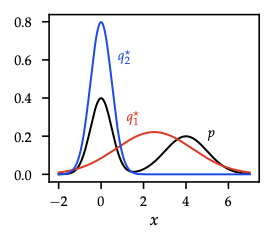
Figure 15: Forward (red) versus reverse (blue) KL: forward KL spreads mass to cover \(p\), reverse KL locks onto the closest mode.

Noninformative prior (\(p(\theta)\propto 1\)) ⇒ maximize average log-likelihood + entropy (maximum-entropy principle).

Gradient estimators

Need \(\nabla_{\lambda} \mathcal{L}(q_{\lambda})\).
Score-function estimator (REINFORCE): \[\nabla_{\lambda} \mathbb{E}_q[f(\theta)] = \mathbb{E}_q[f(\theta)\nabla_{\lambda}\log q_{\lambda}(\theta)],\] general but high variance ⇒ use baselines/control variates (Lemma 5.6).
Reparameterization trick (Thm. 5.8): express \(\theta=g(\varepsilon;\lambda)\) with \(\varepsilon\sim p(\varepsilon)\) independent of \(\lambda\), then \[\nabla_{\lambda} \mathbb{E}_q[f(\theta)] = \mathbb{E}_{\varepsilon}[\nabla_{\lambda} f(g(\varepsilon;\lambda))].\] For Gaussian \(q_{\lambda}\): \(\theta=\mu+L\varepsilon\), \(\varepsilon\sim\mathcal{N}(0,I)\). Backbone of black-box VI, VAEs, and policy gradients with reparameterized actions.

Practical VI recipe

Choose family \(q_{\lambda}(\theta)\) (mean-field Gaussian, full-covariance, normalizing flows, etc.).
Write ELBO; split analytic terms (KL for Gaussians) vs MC terms (expected log-likelihood).
Estimate gradients using reparameterization or score-function + baselines.
Optimize with SGD/Adam; optionally natural gradients (mirror descent under KL geometry).

Predictive inference

Approximate predictive \(p(y^*\mid x^*,\mathcal{D}) \approx \int p(y^*\mid x^*,\theta)q(\theta)d\theta\) via Monte Carlo.
For GLM with Gaussian \(q\): integrate out weights analytically to 1-D latent \(f^*\sim\mathcal{N}(\mu^\top x^*, x^{*\top}\Sigma x^*)\), then compute \(\int p(y^*\mid f^*)\mathcal{N}\) (e.g., logistic regression uses Gauss-Hermite quadrature or probit approximation).

Information-theoretic view

Figure 16: Probability space (left) and the corresponding surprise space obtained via the \(-\log\) transform.

Free energy \(F(q)=-\mathcal{L}(q)=\mathbb{E}_q[\mathcal{S}(p(\mathcal{D},\theta))] - \mathcal{H}(q)\).
Minimizing \(F\) trades “energy” (data fit) against entropy (spread). The same curiosity vs conformity principle shows up in max-entropy RL and exploration bonuses.

Choice of variational family

Mean-field Gaussian ⇒ two parameters per latent; cheap but ignores correlations (underestimates variance).
Full-covariance Gaussian ⇒ \(\mathcal{O}(d^2)\) params.
Structured families: mixture of Gaussians, low-rank plus diagonal, normalizing flows (invertible transforms) for richer posterior shapes.
Hierarchical priors/hyperpriors: introduce latent hyperparameters \(\eta\), augment \(q(\theta,\eta)\) with factorization.

Connections to later chapters

Score-function estimator = REINFORCE gradient with baselines derived here.
Reparameterization trick reappears in stochastic value gradients and dropout-as-VI.
Free-energy viewpoint parallels entropy-regularized RL and active-learning acquisition design.

Markov Chain Monte Carlo

Overview

Turn posterior sampling into Markov-chain design for cases where variational approximations fall short.

Figure 17: Directed graphical model of a Markov chain. The random variable \(X_{t+1}\) is conditionally independent of the random variables \(X_{0:t-1}\) given \(X_t\).

Figure 18: Transition graphs of Markov chains: (1) is not ergodic as its transition diagram is not strongly connected; (2) is not ergodic for the same reason; (3) is irreducible but periodic and therefore not ergodic; (4) is ergodic with stationary distribution \(\pi(1) = \frac{2}{3}, \pi(2) = \frac{1}{3}\).

Markov-chain preliminaries

Homogeneous chain with transition kernel \(P(x'\mid x)\); \(k\)-step transition \(P^k\).
Stationary distribution \(\pi\) solves \(\pi^\top P = \pi^\top\). If chain is irreducible and aperiodic (ergodic), \(q_t\to\pi\) for any start (Fundamental theorem; see Figure 18 ).
Detailed balance \(\pi(x)P(x'\mid x)=\pi(x')P(x\mid x')\) suffices for stationarity (reversibility).
Distance to stationarity measured in total variation \(\|q_t-\pi\|_{\mathrm{TV}}\); mixing time \(\tau_{\mathrm{mix}}(\epsilon)\) ≈ steps to get within \(\epsilon\).

Metropolis–Hastings (MH)

Goal: target density \(p(x)=q(x)/Z\) (unnormalized \(q\) known).
Proposal \(r(x'\mid x)\); accept with \[\alpha(x'\mid x)=\min\left\{1,\frac{q(x')r(x\mid x')}{q(x)r(x'\mid x)}\right\}.\]
Ensures detailed balance w.r.t. \(p\).
Tuning: poor proposals ⇒ slow mixing (random walk). Adaptive schemes adjust step size to hit desired acceptance (≈0.234 in high-dims for isotropic random walk).

Gradient-informed proposals

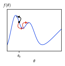
MALA: \(x' = x + \tfrac{\epsilon^2}{2}\nabla\log q(x) + \epsilon\xi\) (Langevin step) then MH accept; leverages gradient, useful in high dimension.
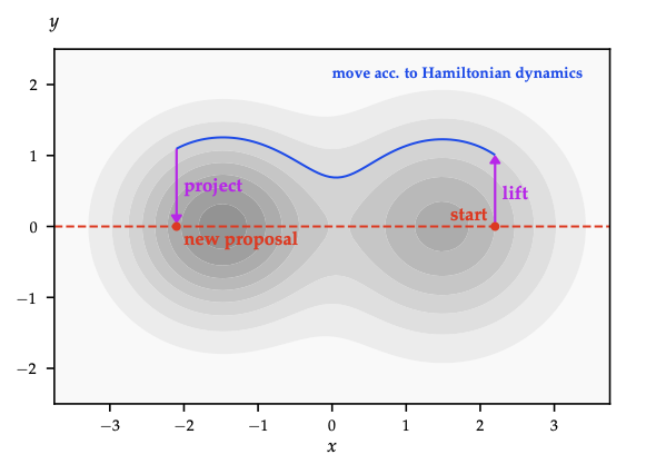
HMC: introduce momentum \(p\sim\mathcal{N}(0,M)\), simulate Hamiltonian dynamics, accept via MH. Long, low-rejection moves reduce random walk behaviour; requires gradient of \(\log q\).
Riemannian manifold HMC: adapt metric to local curvature.

Figure 19: Metropolis–Hastings proposes uninformed jumps; Langevin dynamics follows the gradient of \(f(\theta)\) for more directed moves.

Figure 20: Hamiltonian Monte Carlo lifts states into \((x,y)\) space, simulates Hamiltonian dynamics, and projects back to propose distant points with high acceptance.

Gibbs sampling

Cycle through coordinates (or blocks): sample \(x_i \sim p(x_i\mid x_{-i})\).
Special case of MH with unit acceptance. Works when all conditionals easy; order can be fixed or random (random scan preserves detailed balance).
Block Gibbs improves mixing when variables correlated.

Practical workflow

Initialize (multiple chains if possible).
Burn-in until diagnostics (trace plots, potential scale reduction \(\hat{R}\)) stabilize.
Collect samples, optionally thin to reduce storage (does not improve ESS).
Estimate expectations via Monte Carlo averages; report Monte Carlo error using ESS or batch means.

Energy interpretation

Target \(p(x) \propto e^{-E(x)}\) with energy \(E(x)=-\log q(x)\).
Random-walk MH explores energy landscape slowly; Langevin/HMC follow gradient/level sets ⇒ faster exploration.
Simulated tempering / parallel tempering mix chains at different temperatures to escape local modes.

When to choose MCMC

High-fidelity posterior samples needed (e.g., small models with multimodality) and gradient evaluations affordable.
Combine with VI: use VI for initialization, then MCMC for refinement (e.g., Laplace+MCMC).
Expensive in high dimension; mixing diagnostics essential.

MCMC keeps normalization outside the loop; designing good proposals is the art. Understanding irreducibility, acceptance ratios, and diagnostics is crucial before scaling to Bayesian deep learning or world-model uncertainty.

Bayesian Deep Learning

Overview

Aim: extend Bayesian linear ideas to neural nets, quantify both epistemic/aleatoric uncertainty, and keep models calibrated. Techniques here fuel VI with neural nets, dropout-as-inference, ensembles, and RL exploration bonuses later.

Figure 21: Computation graph of a feed-forward neural network with two hidden layers.

From MAP to Bayesian neural nets

Deterministic NN: \(f(x;\theta)=W_L\varphi(W_{L-1}\cdots\varphi(W_1 x))\).
Likelihood for regression: \(y\mid x,\theta\sim\mathcal{N}(f(x;\theta),\sigma_n^2)\). MAP corresponds to weight decay (Gaussian prior \(\mathcal{N}(0,\sigma_p^2I)\)).
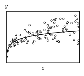
Heteroscedastic likelihood: two-headed output \((\mu(x), \log\sigma^2(x))\) with \(y\mid x,\theta\sim\mathcal{N}(\mu(x),\sigma^2(x))\). Encourages model to learn input-dependent aleatoric noise.

Figure 22: Example of input-dependent (heteroscedastic) noise: variability grows with the magnitude of the inputs.

Variational inference (Bayes by Backprop)

Variational family: factorized Gaussian \(q_\lambda(\theta)=\prod_j \mathcal{N}(\mu_j,\sigma_j^2)\).
ELBO: \[\mathcal{L}(\lambda)=\mathbb{E}_{q_\lambda}[\log p(\mathcal{D}\mid\theta)] - \operatorname{KL}(q_\lambda\|p(\theta)).\]
Use reparameterization \(\theta=\mu+\sigma\odot\varepsilon\), \(\varepsilon\sim\mathcal{N}(0,I)\) to obtain low-variance gradients.
Predictions: Monte Carlo average \(\tfrac{1}{M}\sum_{m}p(y^*\mid x^*,\theta^{(m)})\) with \(\theta^{(m)}\sim q_\lambda\).
SWA/SWAG: collect SGD iterates \(\{\theta^{(t)}\}\), compute empirical mean/covariance, sample Gaussian weights at test time — cheap posterior approximation.

Dropout, dropconnect, masksembles

Dropout: randomly zero activations; dropconnect: randomly zero weights. Gal & Ghahramani: interpret as variational posterior \(q_j(\theta_j)=p\,\delta_0+(1-p)\,\delta_{\lambda_j}\).

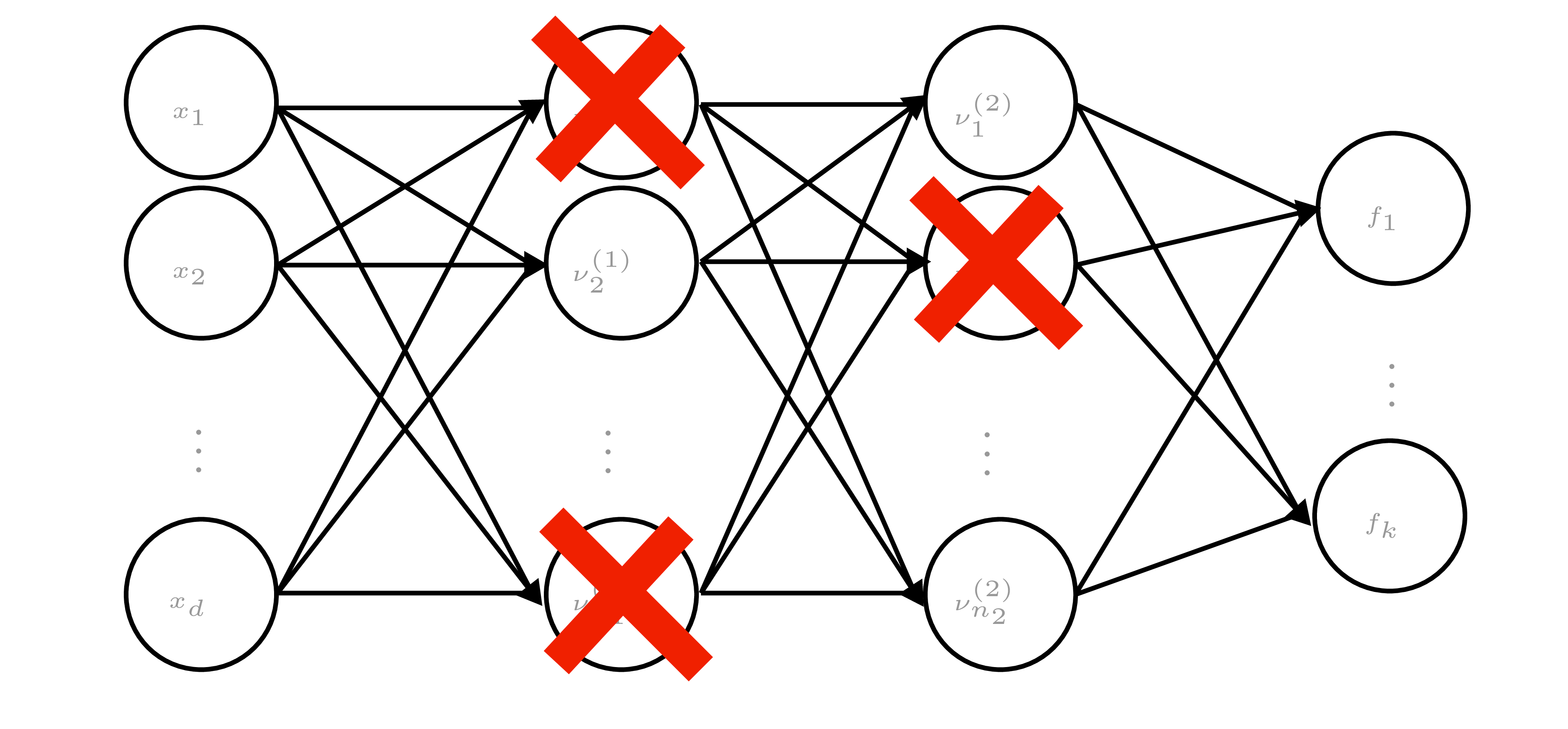
Figure 23: Masksembles cycle through a fixed set of dropout masks with limited overlap to reduce correlation between subnetworks.

Training objective (with weight decay) = ELBO for this \(q_j\). Prediction requires MC dropout (sample masks at test time to capture epistemic uncertainty).
Masksembles: use fixed set of masks with controlled overlap to reduce correlation between subnets.

Probabilistic ensembles

Train \(m\) models \(\{\theta^{(i)}\}\) (bootstrapped data or random init). Predictive distribution \(\approx\tfrac{1}{m}\sum_i p(y^*\mid x^*,\theta^{(i)})\).
Mix with other approximations: e.g., each member uses SWAG or Laplace to yield mixture-of-Gaussians posterior.
Empirical success in OOD detection, uncertainty calibration, and model-based RL.

Calibration diagnostics and fixes

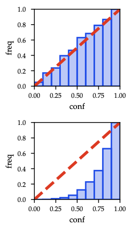
Figure 24: Reliability diagram comparing predicted confidence to empirical accuracy.

As shown in Figure 24, perfect calibration lies on the diagonal; shaded bars mark empirical accuracy gaps.

A model is calibrated if predicted confidence matches empirical accuracy.
Metrics: expected calibration error (ECE), maximum calibration error (MCE).
Techniques:
1. Histogram binning: map each confidence bin to empirical frequency.
2. Isotonic regression: learn monotone piecewise-constant mapping.
3. Platt scaling: fit sigmoid \(\sigma(a z + b)\) to logits.
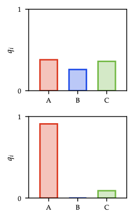
4. Temperature scaling (below): special case (\(b=0\)) adjusting sharpness without changing argmax.
Evaluate on held-out validation set; essential when using uncertainty for decision-making (e.g., safe RL).

Figure 25: Effect of temperature scaling: higher \(T\) spreads probability mass across classes, lower \(T\) concentrates it on the top choice.

Key takeaways

MAP yields point predictions only; capturing epistemic uncertainty requires VI, dropout-as-VI, SWAG, or ensembles.
MC averaging at test time is non-negotiable when using stochastic approximations.
Proper calibration is necessary before feeding uncertainties into downstream tasks (active learning, Bayesian optimization, safe RL).

Active Learning

Overview

Turn posterior uncertainty into data-acquisition policies. Mutual information + submodularity justify greedy sampling.

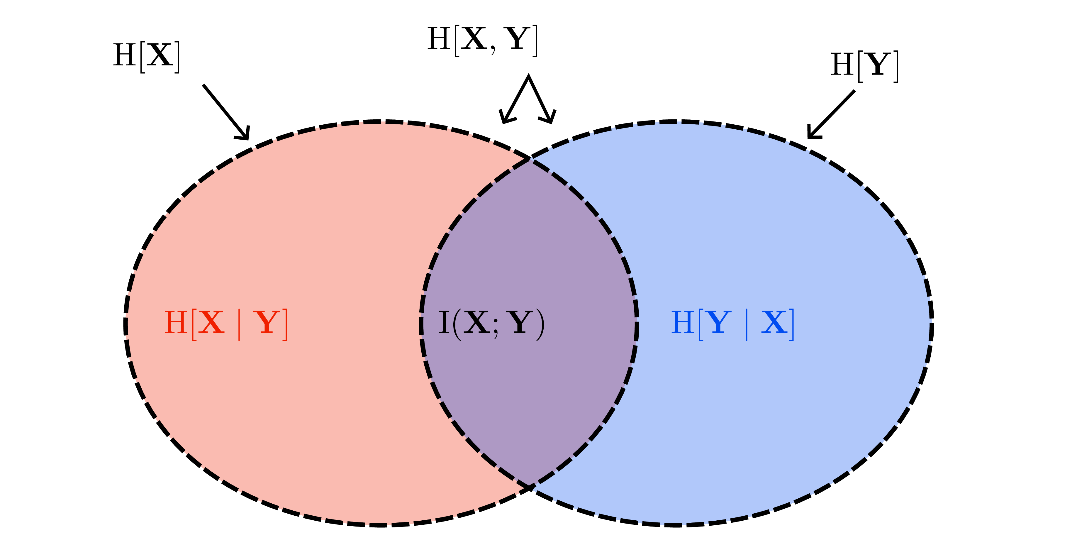
Figure 26: Mutual information decomposed as overlapping entropy of \(X\) and \(Y\).

Entropy and mutual information recap

Conditional entropy \(H(X\mid Y)=\mathbb{E}[-\log p(X\mid Y)]\) measures expected residual uncertainty after observing \(Y\); “information never hurts”: \(H(X\mid Y)\le H(X)\).
Mutual information \(I(X;Y)=H(X)-H(X\mid Y)=H(Y)-H(Y\mid X)\) quantifies expected entropy reduction.
Conditional MI \(I(X;Y\mid Z)\) supports incremental updates; interaction information distinguishes redundancy vs synergy.
Data processing inequality: \(X\to Y\to Z\) ⇒ \(I(X;Z)\le I(X;Y)\) — ensures that coarsening observations cannot increase utility.

MI-based acquisition

Observations \(y_x = f(x) + \varepsilon_x\), \(\varepsilon_x\sim\mathcal{N}(0,\sigma_n^2)\).
Utility of subset \(S\subseteq\mathcal{X}\): \[I(S)=I(f_S; y_S) = H(f_S) - H(f_S\mid y_S).\]
Marginal gain when adding \(x\): \[\Delta_I(x\mid S) = I(f_x; y_x\mid y_S) = H(y_x\mid y_S) - H(\varepsilon_x).\] First term = posterior predictive entropy at \(x\), second = irreducible noise.
For Gaussian models (e.g., GP surrogate) \(H(y_x\mid y_S)\) has closed form via posterior variance.

Submodularity & greedy optimality

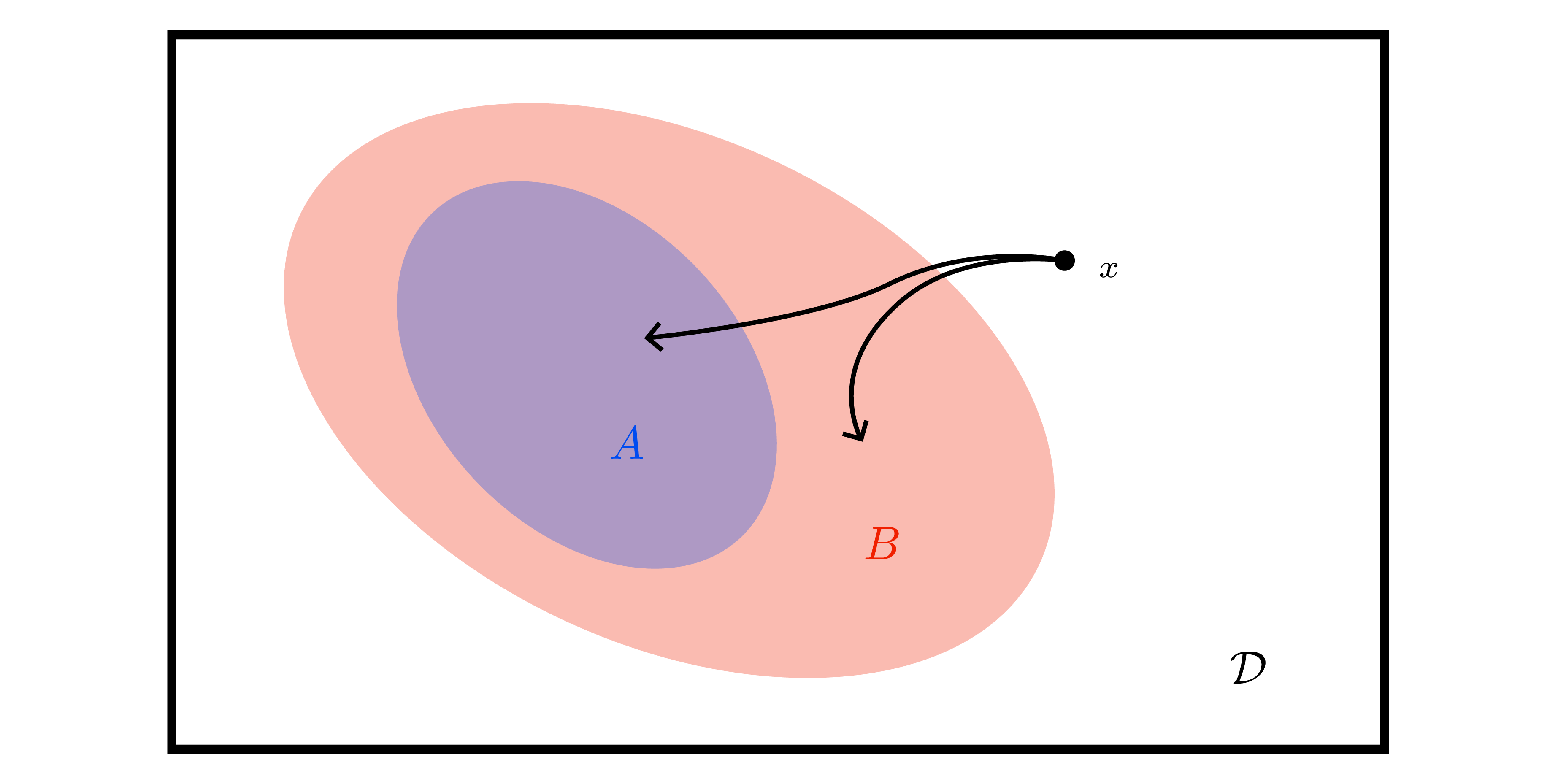
Figure 27: Monotone submodularity. The effect of adding \(x\) to the smaller set \(A\) is larger than the effect of adding \(x\) to the larger set \(B\).

Function \(F\) is submodular if \(\Delta_F(x\mid A) \ge \Delta_F(x\mid B)\) whenever \(A\subseteq B\) — discrete analogue of concavity.
Mutual information \(I(S)\) is monotone submodular when observations are conditionally independent given latent \(f\) (true for GP with Gaussian noise, LVMs, etc.). Ergo greedy selection (Argmax of \(\Delta_I\)) is \((1-1/e)\)-approximate optimal (Nemhauser et al.).
Absence of synergy corresponds to submodularity (Exercise 8.3): if learning one point never increases the value of another, greedy works.

Greedy active learning loop

Maintain posterior over \(f\) (GP or Bayesian NN).
For each candidate \(x\), compute predictive entropy \(H(y_x\mid y_S)\) and marginal gain \(\Delta_I(x\mid S)\).
Select \(x^{\star}=\arg\max_x \Delta_I(x\mid S)\) (or pick \(k\) highest for batch selection).
Query label, update posterior, repeat until budget exhausted.

Variants & practical notes

Batch active learning: use submodular maximization with lazy evaluation or approximate greedy.
Diversity heuristics: when posterior approximations cheap, combine MI with coverage or kernel herding.
Non-Gaussian likelihoods: use MC estimates of entropy/MI (requires VI or Laplace approximations for tractable gradients).
Noisy annotation costs: weigh MI by cost or expected improvement per time.

Active learning is curiosity formalized: reduce epistemic uncertainty fastest while respecting label budgets. The same MI machinery powers Bayesian optimization and model-based RL exploration bonuses.

Bayesian Optimization

Overview

Black-box optimization with a probabilistic surrogate (typically a Gaussian process). Balances exploration vs exploitation via acquisition functions while connecting to bandit intuition and RL planning.

Figure 28: Contour plots of UCB (with \(\beta_t=0.75\)), PI, and EI as functions of \(\Delta_t\) and \(\sigma_t\); brighter colors mark larger acquisition values.

As shown in Figure 28, PI, EI, and UCB respectively focus exploitation vs exploration for a 2D Branin-like surface.

Problem setup

Unknown objective \(f:\mathcal{X}\to\mathbb{R}\); observations \(y_t = f(x_t) + \varepsilon_t\), \(\varepsilon_t\sim\mathcal{N}(0,\sigma_n^2)\).
Surrogate: GP posterior \((\mu_t(x),\sigma_t^2(x))\) after \(t\) queries.
Acquisition \(a_t(x)\) selects next query \(x_{t+1}=\arg\max_x a_t(x)\).
Trade-off: exploration (high \(\sigma_t\)) vs exploitation (high \(\mu_t\)).

Upper Confidence Bound (UCB)

Optimism in face of uncertainty (OFU): \[x_{t+1}=\arg\max_x \mu_t(x)+\beta_{t+1}^{1/2}\,\sigma_t(x).\]
\(\beta_t\) controls confidence width; choose schedule to guarantee \(f(x)\in[\mu_t(x)\pm\beta_t^{1/2}\sigma_t(x)]\) with high prob.
Bayesian setting: \(\beta_t = 2\log\frac{|\mathcal{X}|\pi^2 t^2}{6\delta}\) (finite domain). Frequentist: \(\beta_t= B + 4\sigma_n\sqrt{\gamma_{t-1}+1+\ln(1/\delta)}\) when \(f\) bounded in RKHS (Theorem 9.3).
Regret bound \(\mathcal{O}(\sqrt{T\beta_T\gamma_T})\) where \(\gamma_T\) is information gain of kernel (RBF: \(\gamma_T=\tilde{\mathcal{O}}((\log T)^{d+1})\)).

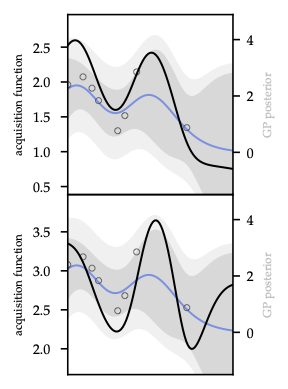
Figure 29: Upper-confidence bound acquisition scores for \(\beta=0.25\) (left) and \(\beta=1\) (right).

As Figure 29 illustrates, confidence tubes widen on sparse data, making the optimism term explicit.

Improvement-based acquisition

Maintain incumbent best \(\hat{f}_t=\max_{\tau\le t} y_\tau\).
Probability of improvement (PI): \[a_t^{\mathrm{PI}}(x)=\Phi\Big(\frac{\mu_t(x)-\hat{f}_t-\xi}{\sigma_t(x)}\Big)\] with exploration parameter \(\xi\ge0\) (larger \(\xi\) encourages exploration).
Expected improvement (EI): \[a_t^{\mathrm{EI}}(x) = (\mu_t(x)-\hat{f}_t-\xi)\Phi(z) + \sigma_t(x)\phi(z),\quad z=\frac{\mu_t(x)-\hat{f}_t-\xi}{\sigma_t(x)}.\] Closed form for Gaussian surrogate; often optimize \(\log\text{EI}\) to avoid flatness.
Both rely on Gaussian predictive distribution; for non-Gaussian surrogates use quadrature or MC.

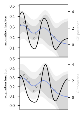
Figure 30: Probability of improvement (PI) and expected improvement (EI) acquisition functions.

As Figure 30 shows, PI saturates once \(\mu_t\) exceeds the incumbent, whereas EI still values high-variance points — the ridge over \(\hat{f}_t\) remains.

Thompson sampling / probability matching

Sample function \(\tilde{f}\sim\mathcal{GP}(\mu_t,k_t)\) and pick \(x_{t+1}=\arg\max_x \tilde{f}(x)\).
Equivalent to sampling from probability of optimality distribution \(\pi(x)=\Pr[\tilde{f}(x)=\max_x \tilde{f}(x)]\).
Implement via random Fourier features or basis projection to draw approximate GP sample.

Exploratory design connections

MI view: \(\Delta_I(x)=\tfrac{1}{2}\log(1+\sigma_t^{-2}(x)\sigma^2_{\varepsilon})\) for GP ⇒ UCB/EI can be seen as MI proxies.
Knowledge gradient / information-directed sampling combine expected reward improvement with information gain.
Acquisition trade-offs often tuned by schedule \(\beta_t\), \(\xi_t\), or entropy regularization.

Optimization of acquisition

Non-convex; in low \(d\) use dense grids + local optimization, in higher \(d\) use multi-start gradient ascent, evolutionary strategies, or sample-evaluate heuristics.
Warm-start new acquisition maximization from previous maximizers.
Constraints: handle by penalizing infeasible points or modeling constraint GP.

Practicalities

Hyperparameters: re-optimize GP kernel parameters via marginal likelihood after each few observations; rely on priors to avoid overfitting small data.
Noise estimation: inaccurate noise variance breaks UCB/EI calibration.
Batch BO: choose multiple points per round via fantasizing or \(q\)-EI/TS.
Termination: when acquisition near zero or budget exhausted.

Links forward

UCB-style optimism echoes exploration bonuses in RL.
Thompson sampling in model space mirrors ensemble sampling strategies for world models.
Entropy-based acquisition sets the stage for maximum-entropy RL.

Markov Decision Processes

Overview

Anchor chapter for all RL work: tighten the core equations, understand the exact-solution algorithms, and know how partial observability folds back into the same machinery.

Figure 31: Graphical model of an MDP: states \(X_t\) transition under actions \(A_t\).

Setup recap

Finite MDP \(\mathcal{M}=(\mathcal{X},\mathcal{A},p,r,\gamma)\) with discount \(\gamma\in[0,1)\); discounted payoff \(G_t=\sum_{m\ge 0}\gamma^m R_{t+m}\).
Stationary policy \(\pi(a\mid x)\) induces Markov chain with transition matrix \(P^\pi(x'\mid x)=\sum_a \pi(a\mid x)p(x'\mid x,a)\) and expected one-step reward \(r^\pi(x)=\sum_a \pi(a\mid x)r(x,a)\).
Value functions:
- \(v^\pi(x)=\mathbb{E}_\pi[G_t\mid X_t=x]\).
- \(q^\pi(x,a)=r(x,a)+\gamma\sum_{x'} p(x'\mid x,a)v^\pi(x')\).
- Advantage \(a^\pi(x,a)=q^\pi(x,a)-v^\pi(x)\) (useful later).

Bellman identities + contraction view

Expectation form: \(v^\pi = r^\pi + \gamma P^\pi v^\pi\).
Matrix solution: \(v^\pi = (I-\gamma P^\pi)^{-1} r^\pi\) whenever \(I-\gamma P^\pi\) invertible (always for \(\gamma<1\)).
Optimality form:
- \(v^*(x)=\max_a\big[r(x,a)+\gamma\sum_{x'}p(x'\mid x,a)v^*(x')\big]\).
- \(q^*(x,a)=r(x,a)+\gamma\sum_{x'}p(x'\mid x,a)\max_{a'}q^*(x',a')\).
Contraction property (Banach fixed point): operators \(B^\pi v=r^\pi+\gamma P^\pi v\) and \(B^* v = \max_a \big[r(x,a)+\gamma\sum_{x'}p(x'\mid x,a)v(x')\big]\) both contract in \(\|\cdot\|_\infty\) with modulus \(\gamma\). ⇒ Fixed point unique and iterates converge geometrically (\(\|v_{t}-v^\pi\|_\infty\le\gamma^t\|v_0-v^\pi\|_\infty\)).

Greedy policies and monotone improvement

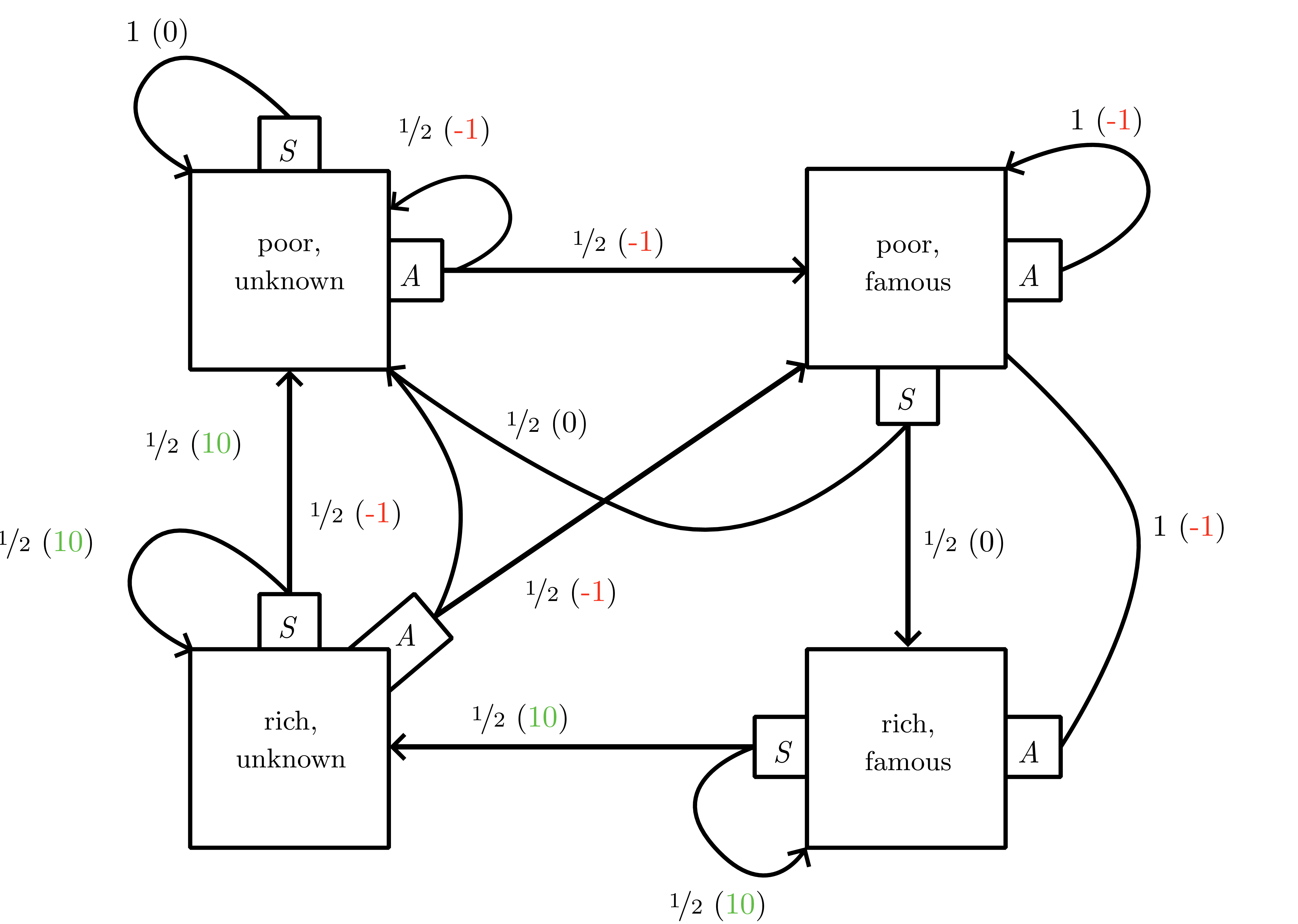{#fig-10-mdp_example fig-align=“center” width=“80%”rich and famous” MDP: saving yields short-term reward but advertising unlocks future high-payoff states.”}

Greedy wrt \(v\): \(\pi_v(x)=\arg\max_a r(x,a)+\gamma\sum_{x'}p(x'\mid x,a)v(x')\) (same as \(\arg\max_a q(x,a)\)).
Policy improvement theorem: \(v^{\pi_v}\ge v\); strict for some \(x\) unless \(v\equiv v^*\). Use this to define partial order over policies and establish existence of deterministic \(\pi^*\).

Exact solution algorithms

Policy iteration (Alg. 10.1)
1. Policy evaluation: solve \((I-\gamma P^{\pi_t}) v^{\pi_t} = r^{\pi_t}\) (direct solve \(\mathcal{O}(|\mathcal{X}|^3)\) or iterative).
2. Improvement: \(\pi_{t+1}=\pi_{v^{\pi_t}}\).
- Monotone convergence (Lemma 10.7); terminates in finitely many steps because only finitely many deterministic policies exist. Linear convergence bound \(\|v^{\pi_t}-v^*\|_\infty\le\gamma^t\|v^{\pi_0}-v^*\|_\infty\).
- Linear programming formulation (Bellman inequalities) gives alternative derivation and underpins reward shaping (see reward_modification exercise).
Value iteration (Alg. 10.2)
- Start with optimistic \(v_0(x)=\max_a r(x,a)\) (or zero) and iterate \(v_{t+1}=B^* v_t\).
- Converges to \(v^*\) asymptotically; \(\epsilon\)-optimal after \(\mathcal{O}(\log(\epsilon^{-1})/(1-\gamma))\) sweeps. Each sweep costs \(\mathcal{O}(|\mathcal{X}||\mathcal{A}|)\) if transitions sparse.
- Dynamic-programming interpretation: \(v_t\) = optimal return for \(t\)-step horizon + terminal reward \(0\).
Asynchronous variants: Gauss-Seidel or prioritized sweeping still contract; practical for large tables.

POMDPs and belief MDPs

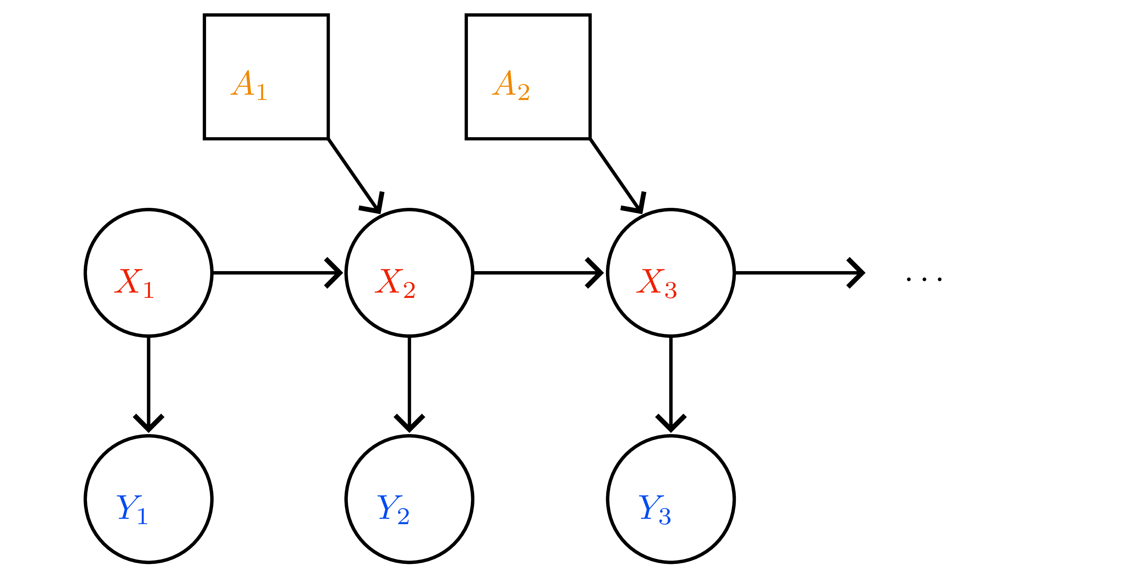
Figure 32: Graphical model of a POMDP with latent states \(X_t\), observations \(Y_t\), and actions \(A_t\).

POMDP \(=(\mathcal{X},\mathcal{A},\mathcal{Y},p,o,r)\); observation model \(o(y\mid x)\).
Filtering update (Bayes):
- Predict: \(\bar{b}_{t+1}(x)=\sum_{x'}p(x\mid x',a_t)b_t(x')\).
- Update: \(b_{t+1}(x)=\frac{o(y_{t+1}\mid x)\bar{b}_{t+1}(x)}{\sum_{x''}o(y_{t+1}\mid x'')\bar{b}_{t+1}(x'')}\).
Belief MDP: state space is simplex \(\Delta^{\mathcal{X}}\), reward \(\rho(b,a)=\sum_x b(x)r(x,a)\), transition kernel \(\tau(b'\mid b,a)=\sum_{y} \mathbf{1}\{b' = \text{BeliefUpdate}(b,a,y)\} \Pr(y\mid b,a)\).
Exact planning infeasible (continuous state). Motivates approximate solvers (point-based value iteration, particle filters) later; Kalman filtering handles the linear-Gaussian case.

Safety, reward shaping, and convergence notes

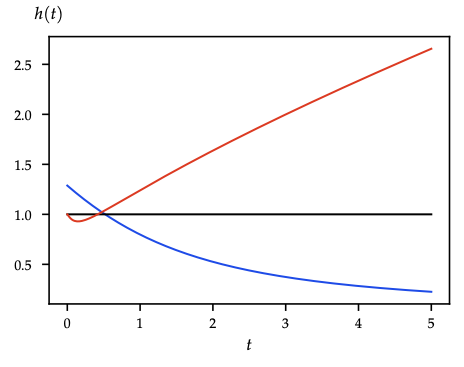
Reward scaling (\(r' = \alpha r\)) leaves optimal policy invariant; additive constants may change optimal policy (exercise reward_modification). Potential-based shaping \(f(x,x')=\gamma\phi(x')-\phi(x)\) preserves optimal policies and avoids clever gamers exploiting hacked bonuses (see simulated “reward gaming” below).

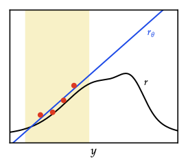
Figure 33: Reward gaming: the learned proxy reward can be exploited outside the feedback region.

Mixing-time perspective: fundamental theorem of ergodic Markov chains (see Figure 18 ) ensures convergence of state distribution under stationary policy; visualize waiting times to revisit states via the coupon-collector-style decay below.

Figure 34: Coupon-collector style decay of expected waiting times before a state is revisited.

Cross-links for later chapters

Discounted payoff definition reused in all subsequent RL chapters.
Greedy-with-respect-to-value operator \(\pi_v\) reappears in policy iteration style updates for both tabular and approximate RL.
Belief-state construction is the conceptual bridge to latent world models and particle filtering in model-based RL.

Tabular Reinforcement Learning

Overview

Bridge from exact planning to learning in unknown MDPs. Keep the exploration logic, convergence preconditions, and where optimism pays off.

Figure 35: In reinforcement learning, an agent interacts with its environment in a sequence of rounds. After playing an action~\(a_t\), it observes rewards~\(r_t\) and its new state~\(x_{t+1}\). The agent then uses this information to learn how to act to maximize reward.

Data model and independence

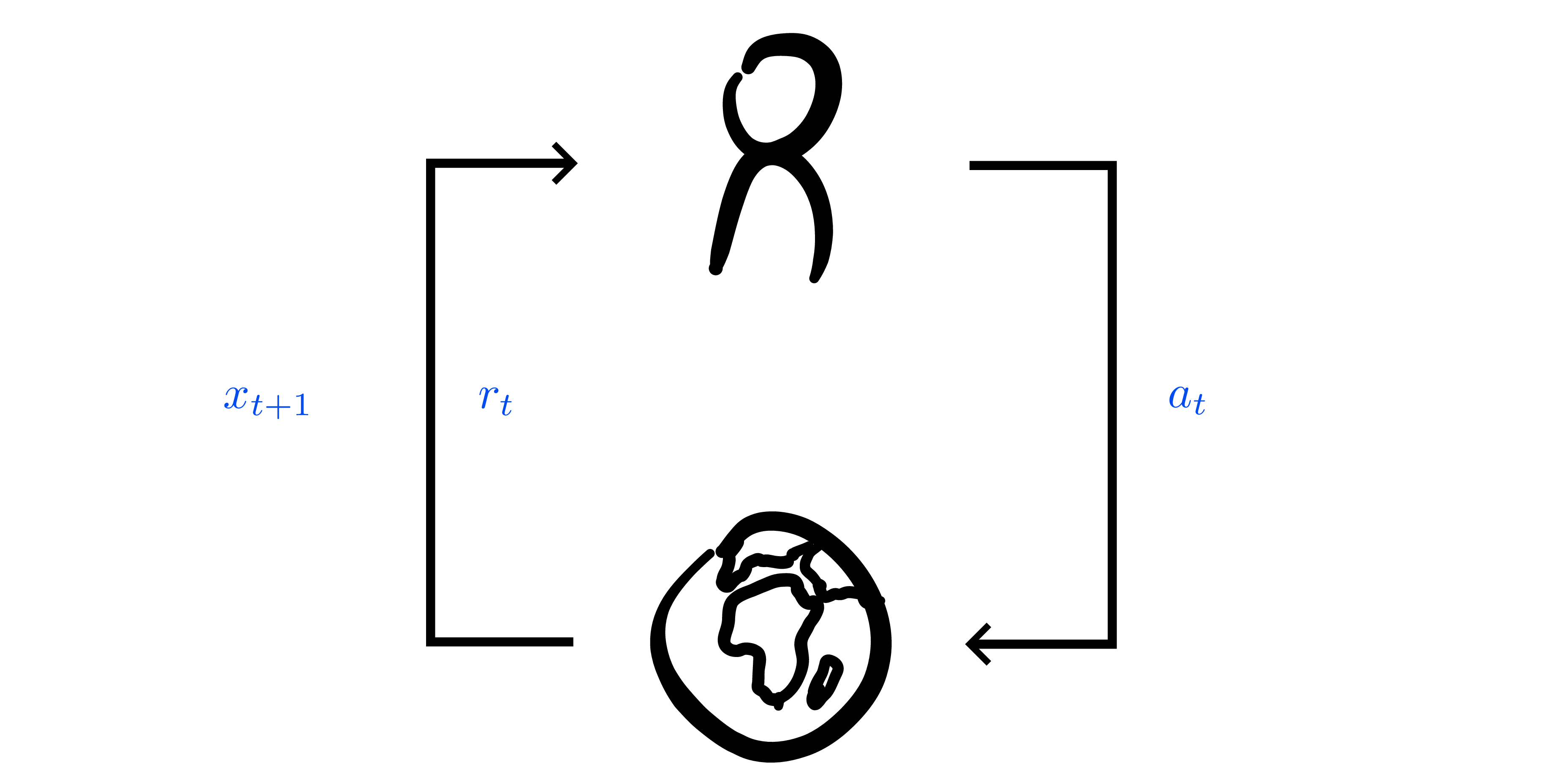
Trajectories \(\tau=(x_0,a_0,r_0,x_1,\dots)\) with transitions drawn from unknown \(p\) and \(r\).
Conditional independence (Eq. 11.2): repeated visits to the same \((x,a)\) give IID samples of \(p(\cdot\mid x,a)\) and \(r(x,a)\) ⇒ Hoeffding + LLN applicable per state-action.
Objective: learn policy maximizing discounted return \(G_0\) without prior model access.

Model-based tabular control

Empirical model \(\hat{p}(x'\mid x,a)=N(x,a,x')/N(x,a)\), \(\hat{r}(x,a)=\sum r/N(x,a)\).
Monte Carlo control: alternate policy evaluation (episode rollouts) and greedy improvement. Exploration via \(\varepsilon\)-greedy with Robbins–Monro schedule (\(\sum \varepsilon_t=\infty\), \(\sum \varepsilon_t^2<\infty\)) ⇒ GLIE ⇒ almost sure convergence to \(\pi^*\). Softmax/Boltzmann exploration uses Gibbs distribution \(\pi_\lambda(a\mid x)\propto e^{Q(x,a)/\lambda}\) for value-directed exploration.
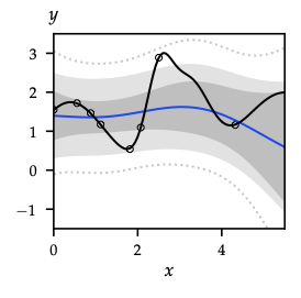
Optimism (\(R_{\max}\)): initialize unknown \((x,a)\) as transitioning to fairy-tale state \(x_s\) with reward \(R_{\max}\) (see below). After \(N(x,a)\) exceeds Hoeffding threshold \(\frac{R_{\max}^2}{2\epsilon^2}\log\frac{2}{\delta}\), replace with empirical model. Guarantees \(\epsilon\)-optimal policy in poly(\(|\mathcal{X}|,|\mathcal{A}|,1/\epsilon,1/\delta\)) steps; chart highlights how bonus intervals shrink with data.

Figure 36: Shrinking confidence bounds as more data is collected.

Figure 37: Illustration of the fairy-tale state of \(R_\mathrm{max}\). If in doubt, the agent believes actions from the state \(x\) to lead to the fairy-tale state \(x^*\) with maximal rewards. This encourages the exploration of unknown states.

Cost: storing dense model \(\mathcal{O}(|\mathcal{X}|^2|\mathcal{A}|)\) + repeatedly solving MDP (policy/value iteration).

Model-free prediction

Monte Carlo evaluation: first-visit / every-visit returns; unbiased but high variance and episode-length dependent.
TD(0): \(V(x) \leftarrow V(x)+\alpha_t\delta_t\) with \(\delta_t=r+\gamma V(x')-V(x)\). Converges almost surely if each state visited infinitely often and \(\alpha_t\) satisfies RM. Generalizes to TD(\(\lambda\)) by using eligibility traces.

On-policy control

SARSA: \(Q(x,a) \leftarrow Q(x,a)+\alpha_t\big(r + \gamma Q(x',a') - Q(x,a)\big)\) where \((x',a')\) drawn from behavior policy. With GLIE exploration and RM step sizes, \(Q\to q^{\pi^*}\) (Theorem 11.4).
Incremental policy-iteration view: evaluate with SARSA, improve greedily (still need exploration noise to avoid collapse).
Actor interpretation: SARSA TD-error \(\delta_t\) is the advantage signal later reused in actor-critic.

Off-policy evaluation and control

Off-policy TD: \(Q(x,a) \leftarrow Q(x,a)+\alpha_t\big(r + \gamma \sum_{a'}\pi(a'\mid x')Q(x',a') - Q(x,a)\big)\) for arbitrary behavior. Enables reuse of logged data.
Q-learning: \(Q(x,a) \leftarrow Q(x,a)+\alpha_t\big(r + \gamma \max_{a'}Q(x',a') - Q(x,a)\big)\).
- Requires all \((x,a)\) sampled infinitely often; \(\alpha_t\) with RM ⇒ almost sure convergence.
- Sample complexity (Even-Dar & Mansour 2003): poly in \(\log |\mathcal{X}|,\log |\mathcal{A}|,1/\epsilon,\log(1/\delta)\).
- Optimistic initialization or \(R_{\max}\)-style bonuses accelerate exploration (precursor to UCB-like deep RL bonuses).
- Coverage assumptions foreshadow importance-sampling corrections later.

Step-size schedules & GLIE condition

Robbins–Monro: \(\alpha_t\ge 0\), \(\sum_t\alpha_t=\infty\), \(\sum_t\alpha_t^2<\infty\) (e.g. \(1/t\), \(1/(1+N_t(x,a))\)).
GLIE (Definition 11.2): ensures infinite exploration + greedy limit, critical for convergence of Monte Carlo control, SARSA, Q-learning.

Exploration heuristics summary

\(\varepsilon\)-greedy: uniform randomization baseline; decays to zero while keeping \(\sum \varepsilon_t = \infty\).
Softmax / Boltzmann: temperature-driven action weighting.
Optimism (R\(_{\max}\), optimistic Q-init): treat unknown as high-value until proven otherwise.
These strategies foreshadow exploration bonuses, entropy regularization, and max-entropy RL.

When to choose which approach

Model-based tabular (with optimistic bonuses) wins on sample efficiency for small MDPs; expensive in memory/compute.
TD/SARSA: incremental, low memory; need on-policy data and exploration schedule.
Q-learning: off-policy, reuses experience replay later (deep RL); sensitive to coverage, step sizes.

Remember: all proofs hinge on (i) every \((x,a)\) visited infinitely often, and (ii) step sizes satisfying RM. These assumptions collapse once we approximate or restrict data, motivating the heavier machinery in Chapters 12–13.

Model-free Approximate RL

Overview

Now we leave the tabular comfort zone. Key aims: reinterpret TD/Q updates as stochastic optimization, understand why deep Q-learning needs stabilizers, tame policy gradient variance, and see how entropy-regularized RL links back to probabilistic inference.

Figure 38: MDP studied in . Each arrow marks a (deterministic) transition and is labeled with \((\text{action},\text{reward})\).

TD/Q as stochastic optimization

Parametrize value/Q with \(\theta\) and fit the Bellman equation in least-squares form.
Per-sample TD loss: \(\ell(\theta)=\tfrac{1}{2}\big(r+\gamma V(x';\theta^-) - V(x;\theta)\big)^2\) with target network \(\theta^-\) frozen for stability; gradient \(\nabla_\theta \ell = (V(x;\theta)-y)\nabla_\theta V(x;\theta)\).
Function approximation + bootstrapping + off-policy = “deadly triad” ⇒ convergence no longer guaranteed, so we need heuristics (replay buffers, target networks, clipping, etc.).

Deep Q-Network (DQN) family

Replay buffer \(\mathcal{D}\) makes samples approximately IID.
Target network updates every \(K\) steps.
Loss: \(\mathcal{L}_{\mathrm{DQN}}=\tfrac{1}{2}\mathbb{E}_{(x,a,r,x')\sim\mathcal{D}}\big[r+\gamma\max_{a'}Q(x',a';\theta^{-})-Q(x,a;\theta)\big]^2\).
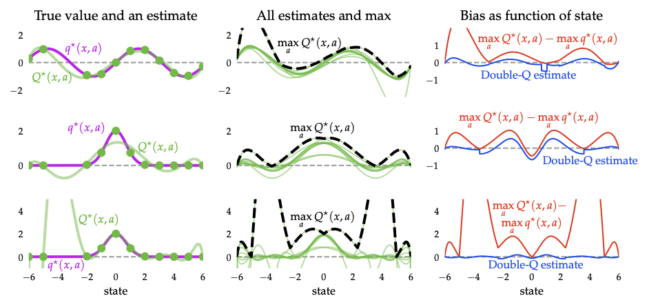
Maximization bias: \(\max\) of noisy estimates overestimates true values. Double DQN fixes this via decoupled action selection/evaluation: target \(r + \gamma Q(x',\arg\max_{a'}Q(x',a';\theta);\theta^{-})\); side-by-side sweep below shows the over-optimism gap.

Figure 39: Maximization bias: greedy Q-learning overestimates values (red), while Double Q-learning (blue) reduces the bias.

Companion tricks: dueling networks, prioritized replay, distributional RL, noisy nets — all to stabilize training or encourage exploration.

Vanilla policy gradients (REINFORCE)

Objective \(J(\varphi)=\mathbb{E}_{\tau\sim\pi_\varphi}\big[\sum_{t\ge0}\gamma^t r_t\big]\).
Score-function gradient (Lemma 12.5): \(\nabla_{\varphi}J = \mathbb{E}_{\tau}\big[\sum_{t} \gamma^t G_{t:T}\,\nabla_{\varphi}\log\pi_{\varphi}(a_t\mid s_t)\big]\).
Baselines (Lemma 12.6): subtract \(b_t\) independent of \(a_t\) (state-dependent baselines yield downstream returns form) to cut variance.
REINFORCE (Alg. 12.2): Monte Carlo gradient ascent; unbiased but high variance, sensitive to learning-rate choice and can stall in local optima.

On-policy actor-critic family

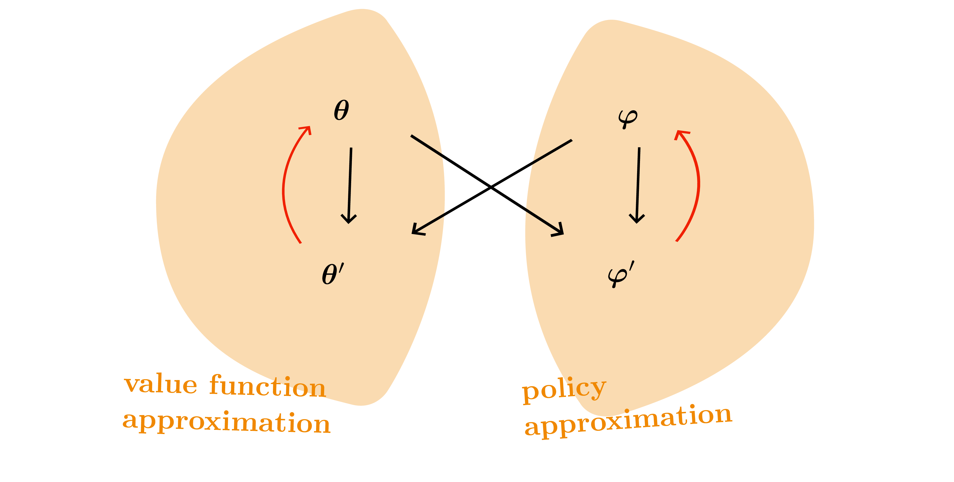
Figure 40: One iteration of an actor–critic method showing the information flow between actor and critic.

Actor = policy \(\pi_{\varphi}\), critic = value/Q \(\hat{Q}_{\theta}\).
Online actor-critic (Alg. 12.3): update actor with \(\hat{Q}_{\theta}\) and critic with SARSA-style TD errors.
Advantage Actor-Critic (A2C): \(\hat{A}_t=r_t+\gamma V(s_{t+1})-V(s_t)\) reduces variance.
Generalized Advantage Estimation (GAE): \(\hat{A}^{\mathrm{GAE}(\lambda)}_t = \sum_{k\ge0}(\gamma\lambda)^k\delta_{t+k}\) with TD errors \(\delta_t=r_t+\gamma V(s_{t+1})-V(s_t)\); tunable bias/variance.
Policy gradient theorem (Eq. 12.24): \(\nabla_{\varphi}J = \frac{1}{1-\gamma}\mathbb{E}_{s\sim\rho_{\pi},a\sim\pi}[A^{\pi}(s,a)\nabla_{\varphi}\log\pi_{\varphi}(a\mid s)]\).
Trust-region methods: TRPO maximizes surrogate under KL constraint; PPO simplifies via clipping or KL penalty; GRPO removes critic using group-relative baselines.

Off-policy actor-critics

Deterministic Policy Gradient (DPG/DDPG): critic trained like DQN, actor updated via \(\nabla_a Q(s,a)\); requires exploration noise.
Twin Delayed DDPG (TD3): twin critics, target policy smoothing, delayed actor updates reduce overestimation.
Stochastic Value Gradients (SVG): use reparameterization for stochastic policies \(a=g(\varepsilon; s,\varphi)\).

Maximum-entropy RL and SAC

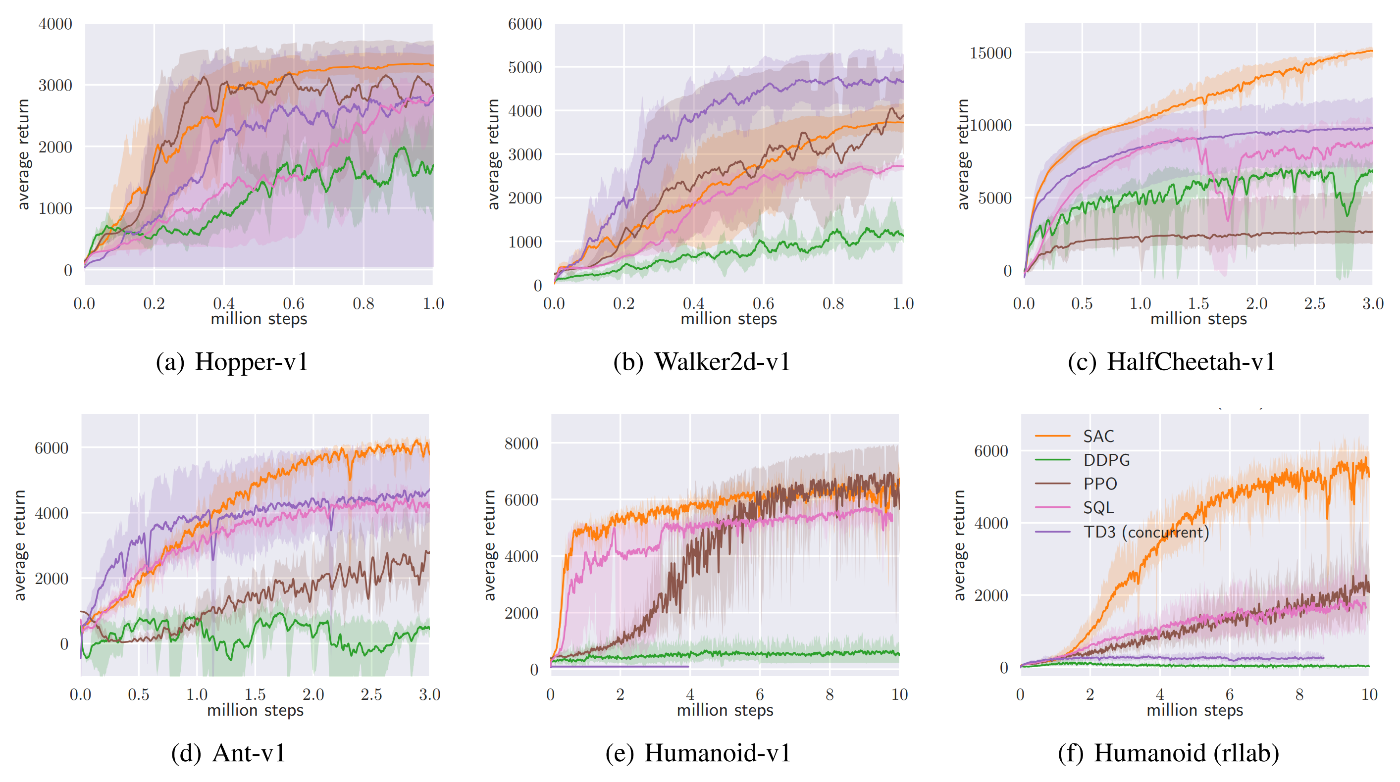
Soft objective \(J_{\alpha}(\pi)=\mathbb{E}[\sum_t\gamma^t(r_t+\alpha\mathcal{H}(\pi(\cdot\mid s_t)))]\).
Soft Bellman backups: \(Q(s,a)=r+\gamma\mathbb{E}_{s'}[V(s')]\), \(V(s)=\alpha\log\int \exp(Q(s,a)/\alpha)da\).
Soft Actor-Critic (SAC): off-policy, stochastic actor; critic matches soft Q, actor minimizes KL to Boltzmann \(\propto\exp((Q-\alpha\log\pi)/\alpha)\); temperature \(\alpha\) tuned to target entropy.
Provides intrinsic exploration and strong sample efficiency in continuous control; entropy plot below shows how higher temperature flattens the implied policy.

Preference-based RL & large models

RLHF/RLAIF pipeline: supervised fine-tune baseline model, learn reward model from preferences, optimize policy via PPO/GRPO with KL penalty to reference.
Objective \(\mathbb{E}[r_{\text{RM}}(y) - \beta\,\mathrm{KL}(\pi\|\pi_{\text{ref}})]\) ↔︎ probabilistic inference with KL regularization.
Critical for aligning large language models; relies on PPO/GRPO mechanics described above.

Practical heuristics & cross-links

Replay + target networks come from DQN and power DDPG/TD3/SAC.
Advantage baselines (A2C/GAE) inherit variance-reduction lemmas from variational inference.
Trust-region/clipping echo KL-constrained optimization in VI.
Entropy bonuses tie back to max-entropy active learning and variational inference.

Every deep RL algorithm is some combination of: replay, target networks, advantage estimates, trust-region regularization, and entropy bonuses. Keep these primitives handy.

Model-based Reinforcement Learning

Overview

Final piece: learn a “world model”, plan through it, and fold epistemic uncertainty into exploration and safety.

Figure 42: Illustration of planning with epistemic uncertainty and Monte Carlo sampling. The agent considers \(m\) alternative ``worlds’’. Within each world, it plans a sequence of actions over a finite time horizon. Then, the agent averages all optimal initial actions from all worlds. Crucially, each world by itself is . That is, its transition model (i.e., the aleatoric uncertainty of the model) is constant.

Outer loop recap

Collect experience with current policy \(\pi\) (real environment).
Learn dynamics \(f_\theta(x,a)\approx p(x'\mid x,a)\) and reward model \(r_\theta(x,a)\) (a.k.a. world model).
Plan/improve policy using the learned model (MPC, trajectory optimization, policy optimization in imagination).
Repeat until convergence or performance threshold.

Reuses familiar value-learning machinery while adding model learning + planning; key benefit is sample efficiency and optional safety analysis.

Planning with the learned model

Figure 43: Illustration of trajectory sampling. High-reward states are shown in brighter colors. The agent iteratively plans a finite number of time steps into the future and picks the best initial action.

Deterministic dynamics

MPC / receding-horizon control: choose horizon \(H\), optimize action sequence \(a_{t:t+H-1}\), apply first action, replan next step.
Objective with terminal bootstrap (Eq. 13.2): \[J_H(a_{t:t+H-1}) = \sum_{\tau=t}^{t+H-1}\gamma^{\tau-t} r(x_\tau,a_\tau) + \gamma^H V(x_{t+H}).\]
Optimization tools: shooting (random sampling), gradient-based (backprop through dynamics), cross-entropy method (CEM) which iteratively reweights samples toward high-return elites.
Special case \(H=1\) recovers the greedy policy from dynamic programming.

Stochastic dynamics

Trajectory sampling / Stochastic Average Approximation: simulate multiple rollouts under candidate action sequence, average returns. Use reparameterization trick to express stochastic dynamics as \(x_{t+1}=g(x_t,a_t;\varepsilon_t)\) for Monte Carlo gradients.
Always replan to mitigate model error accumulation; keep horizon short (5–30 steps) to balance foresight and compounding error.

Learning world models

Deterministic regressors: neural nets, RFF-based GPs, latent linear models.
Probabilistic dynamics: output distribution over next state (e.g., Gaussian with mean/cov). Distinguish aleatoric \(\mathcal{B}(x_{t+1}\mid f,x_t,a_t)\) vs epistemic \(p(f\mid \mathcal{D})\) uncertainty.
Ensembles / BNNs: maintain multiple models \(\{f^{(k)}\}\) (bootstrapped, variational) to approximate epistemic distribution. Used heavily in PETS.
Latent SSMs: PlaNet, Dreamer learn stochastic latent dynamics via variational inference (ELBO). Planner operates in latent space; Dreamer also learns actor/critic in imagination (backprop through latent rollouts).

Planning under epistemic uncertainty

For each sampled model \(f^{(k)}\), perform standard planning (respect aleatoric noise) then average returns/gradients across \(k\). Provides robustness by marginalizing over epistemic uncertainty.
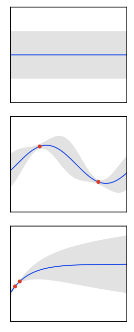
PETS: ensemble of probabilistic networks + MPC via CEM. Handles both uncertainty types; strong sample efficiency on MuJoCo, etc., and the plot below visualizes how epistemic variance concentrates near unexplored regions along candidate plans.
Dreamer/PlaNet: optimize policy/value inside learned latent world; generate imagined rollouts to train actor-critic via policy gradient.

Figure 44: Information gain. The first graph shows the prior. The second graph shows a selection of samples with large information gain (large uncertainty reduction). The third graph shows a selection of samples with small information gain (small uncertainty reduction).

Exploration strategies

Thompson sampling: draw one model sample, plan greedily. Randomizing over models encourages exploration of uncertain regions.
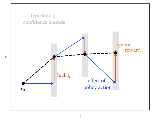
Optimism: introduce “luck” variables \(\eta\) to allow transitions within confidence bounds that favour high reward; ensures optimistic value estimates until uncertainty shrinks.
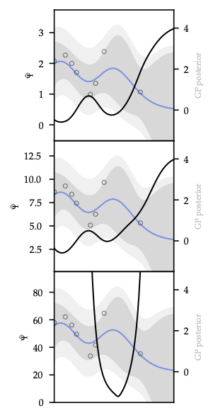
Information-directed sampling: weigh squared regret vs information gain; the heatmap illustrates the ratio used to pick the next rollout.
Safe exploration: propagate uncertainty to enforce chance constraints or reachable sets; combine with MPC for high-probability safety.

Figure 45: Plot of the surrogate information ratio \(\widehat{\Psi}\): IDS selects its minimizer. The first two plots use the “global” information gain measure with \(\beta = 0.25\) and \(\beta = 0.5\), respectively. The third plot uses the “greedy” information gain measure and \(\beta = 1\).

Bridging back to model-free methods

Use world model to generate synthetic data for TD/Q/actor-critic (Dyna style).
Terminal value \(V\) in MPC learned via TD or deep critics.
Planning horizon \(H=1\) reduces to model-free greedy; longer horizons add foresight absent in purely value-based methods.

Practical heuristics

Short horizons + frequent replanning mitigate model error; warm-start optimization from previous solution.
Keep track of epistemic uncertainty (ensembles, Bayesian nets) to decide when additional real data is needed.
Use CEM or evolutionary strategies as robust default for optimizing action sequences.

Safety & guarantees

Confidence sets on dynamics ⇒ safe reachable tubes; combine with MPC to keep agent within safe set despite model error.
Optimistic-yet-safe planners mix optimism (exploration) with reachable-set constraints; HUCRL timeline highlights confidence widening when the agent strays outside proven-safe regions.
Sets stage for constrained RL and control-barrier approaches.