Model-based Reinforcement Learning

Overview

Final piece: learn a “world model”, plan through it, and fold epistemic uncertainty into exploration and safety.

Figure 1: Illustration of planning with epistemic uncertainty and Monte Carlo sampling. The agent considers \(m\) alternative ``worlds’’. Within each world, it plans a sequence of actions over a finite time horizon. Then, the agent averages all optimal initial actions from all worlds. Crucially, each world by itself is . That is, its transition model (i.e., the aleatoric uncertainty of the model) is constant.

Outer loop recap

1. Collect experience with current policy \(\pi\) (real environment).
2. Learn dynamics \(f_\theta(x,a)\approx p(x'\mid x,a)\) and reward model \(r_\theta(x,a)\) (a.k.a. world model).
3. Plan/improve policy using the learned model (MPC, trajectory optimization, policy optimization in imagination).
4. Repeat until convergence or performance threshold.

Reuses familiar value-learning machinery while adding model learning + planning; key benefit is sample efficiency and optional safety analysis.

Planning with the learned model

Figure 2: Illustration of trajectory sampling. High-reward states are shown in brighter colors. The agent iteratively plans a finite number of time steps into the future and picks the best initial action.

Deterministic dynamics

• MPC / receding-horizon control: choose horizon \(H\), optimize action sequence \(a_{t:t+H-1}\), apply first action, replan next step.
• Objective with terminal bootstrap (Eq. 13.2): \[J_H(a_{t:t+H-1}) = \sum_{\tau=t}^{t+H-1}\gamma^{\tau-t} r(x_\tau,a_\tau) + \gamma^H V(x_{t+H}).\]
• Optimization tools: shooting (random sampling), gradient-based (backprop through dynamics), cross-entropy method (CEM) which iteratively reweights samples toward high-return elites.
• Special case \(H=1\) recovers the greedy policy from dynamic programming.

Stochastic dynamics

• Trajectory sampling / Stochastic Average Approximation: simulate multiple rollouts under candidate action sequence, average returns. Use reparameterization trick to express stochastic dynamics as \(x_{t+1}=g(x_t,a_t;\varepsilon_t)\) for Monte Carlo gradients.
• Always replan to mitigate model error accumulation; keep horizon short (5–30 steps) to balance foresight and compounding error.

Learning world models

• Deterministic regressors: neural nets, RFF-based GPs, latent linear models.
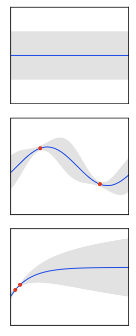
• Probabilistic dynamics: output distribution over next state (e.g., Gaussian with mean/cov). Distinguish aleatoric \(\mathcal{B}(x_{t+1}\mid f,x_t,a_t)\) vs epistemic \(p(f\mid \mathcal{D})\) uncertainty.
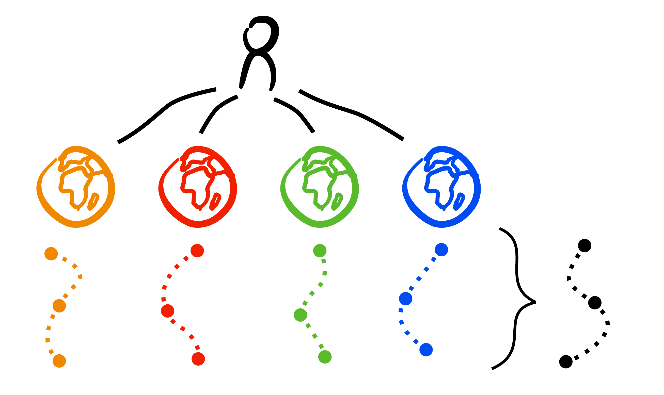
• Ensembles / BNNs: maintain multiple models \(\{f^{(k)}\}\) (bootstrapped, variational) to approximate epistemic distribution. Used heavily in PETS.
• Latent SSMs: PlaNet, Dreamer learn stochastic latent dynamics via variational inference (ELBO). Planner operates in latent space; Dreamer also learns actor/critic in imagination (backprop through latent rollouts).

Planning under epistemic uncertainty

• For each sampled model \(f^{(k)}\), perform standard planning (respect aleatoric noise) then average returns/gradients across \(k\). Provides robustness by marginalizing over epistemic uncertainty.
• PETS: ensemble of probabilistic networks + MPC via CEM. Handles both uncertainty types; strong sample efficiency on MuJoCo, etc., and the plot below visualizes how epistemic variance concentrates near unexplored regions along candidate plans.
• Dreamer/PlaNet: optimize policy/value inside learned latent world; generate imagined rollouts to train actor-critic via policy gradient.

Figure 3: Information gain. The first graph shows the prior. The second graph shows a selection of samples with large information gain (large uncertainty reduction). The third graph shows a selection of samples with small information gain (small uncertainty reduction).

Exploration strategies

• Thompson sampling: draw one model sample, plan greedily. Randomizing over models encourages exploration of uncertain regions.
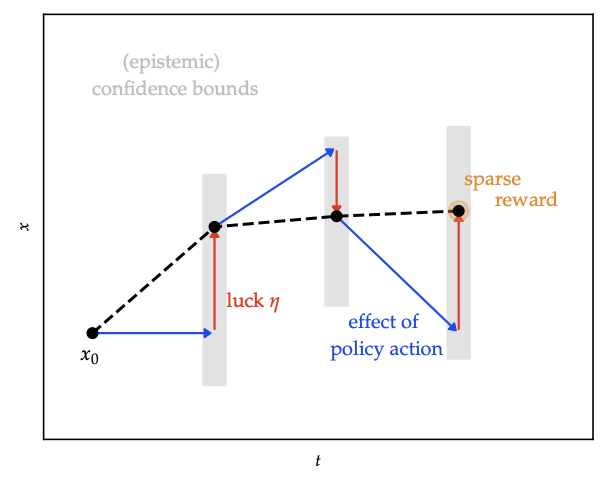
• Optimism: introduce “luck” variables \(\eta\) to allow transitions within confidence bounds that favour high reward; ensures optimistic value estimates until uncertainty shrinks.
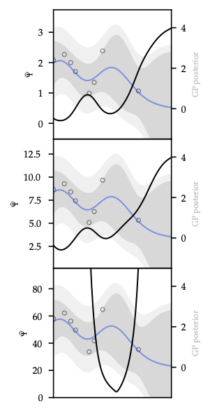
• Information-directed sampling: weigh squared regret vs information gain; the heatmap illustrates the ratio used to pick the next rollout.
• Safe exploration: propagate uncertainty to enforce chance constraints or reachable sets; combine with MPC for high-probability safety.

Figure 4: Plot of the surrogate information ratio \(\widehat{\Psi}\): IDS selects its minimizer. The first two plots use the “global” information gain measure with \(\beta = 0.25\) and \(\beta = 0.5\), respectively. The third plot uses the “greedy” information gain measure and \(\beta = 1\).

Bridging back to model-free methods

• Use world model to generate synthetic data for TD/Q/actor-critic (Dyna style).
• Terminal value \(V\) in MPC learned via TD or deep critics.
• Planning horizon \(H=1\) reduces to model-free greedy; longer horizons add foresight absent in purely value-based methods.

Practical heuristics

• Short horizons + frequent replanning mitigate model error; warm-start optimization from previous solution.
• Keep track of epistemic uncertainty (ensembles, Bayesian nets) to decide when additional real data is needed.
• Use CEM or evolutionary strategies as robust default for optimizing action sequences.

Safety & guarantees

• Confidence sets on dynamics ⇒ safe reachable tubes; combine with MPC to keep agent within safe set despite model error.
• Optimistic-yet-safe planners mix optimism (exploration) with reachable-set constraints; HUCRL timeline highlights confidence widening when the agent strays outside proven-safe regions.
• Sets stage for constrained RL and control-barrier approaches.

Figure 5: Illustration of H-UCRL in a one-dimensional state space. The agent hallucinates that it takes the black trajectory when, in reality, the outcomes of its actions are as shown in blue. The agent can hallucinate to land anywhere within the gray confidence regions (i.e., the epistemic uncertainty in the model) using the luck decision variables \(\eta\). This allows agents to discover long sequences of actions leading to sparse rewards.