Markov Decision Processes
Overview
Anchor chapter for all RL work: tighten the core equations, understand the exact-solution algorithms, and know how partial observability folds back into the same machinery.
Setup recap
- Finite MDP \(\mathcal{M}=(\mathcal{X},\mathcal{A},p,r,\gamma)\) with discount \(\gamma\in[0,1)\); discounted payoff \(G_t=\sum_{m\ge 0}\gamma^m R_{t+m}\).
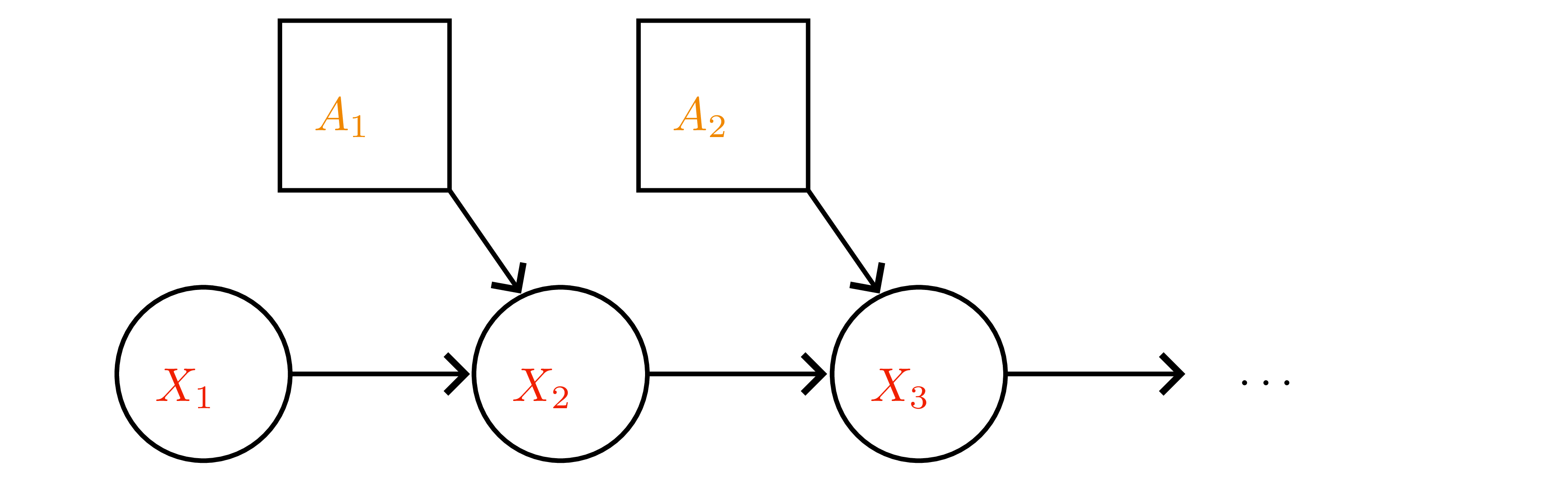
- Stationary policy \(\pi(a\mid x)\) induces Markov chain with transition matrix \(P^\pi(x'\mid x)=\sum_a \pi(a\mid x)p(x'\mid x,a)\) and expected one-step reward \(r^\pi(x)=\sum_a \pi(a\mid x)r(x,a)\).
- Value functions:
- \(v^\pi(x)=\mathbb{E}_\pi[G_t\mid X_t=x]\).
- \(q^\pi(x,a)=r(x,a)+\gamma\sum_{x'} p(x'\mid x,a)v^\pi(x')\).
- Advantage \(a^\pi(x,a)=q^\pi(x,a)-v^\pi(x)\) (useful later).
Bellman identities + contraction view
- Expectation form: \(v^\pi = r^\pi + \gamma P^\pi v^\pi\).
- Matrix solution: \(v^\pi = (I-\gamma P^\pi)^{-1} r^\pi\) whenever \(I-\gamma P^\pi\) invertible (always for \(\gamma<1\)).
- Optimality form:
- \(v^*(x)=\max_a\big[r(x,a)+\gamma\sum_{x'}p(x'\mid x,a)v^*(x')\big]\).
- \(q^*(x,a)=r(x,a)+\gamma\sum_{x'}p(x'\mid x,a)\max_{a'}q^*(x',a')\).
- Contraction property (Banach fixed point): operators \(B^\pi v=r^\pi+\gamma P^\pi v\) and \(B^* v = \max_a \big[r(x,a)+\gamma\sum_{x'}p(x'\mid x,a)v(x')\big]\) both contract in \(\|\cdot\|_\infty\) with modulus \(\gamma\). ⇒ Fixed point unique and iterates converge geometrically (\(\|v_{t}-v^\pi\|_\infty\le\gamma^t\|v_0-v^\pi\|_\infty\)).
Greedy policies and monotone improvement
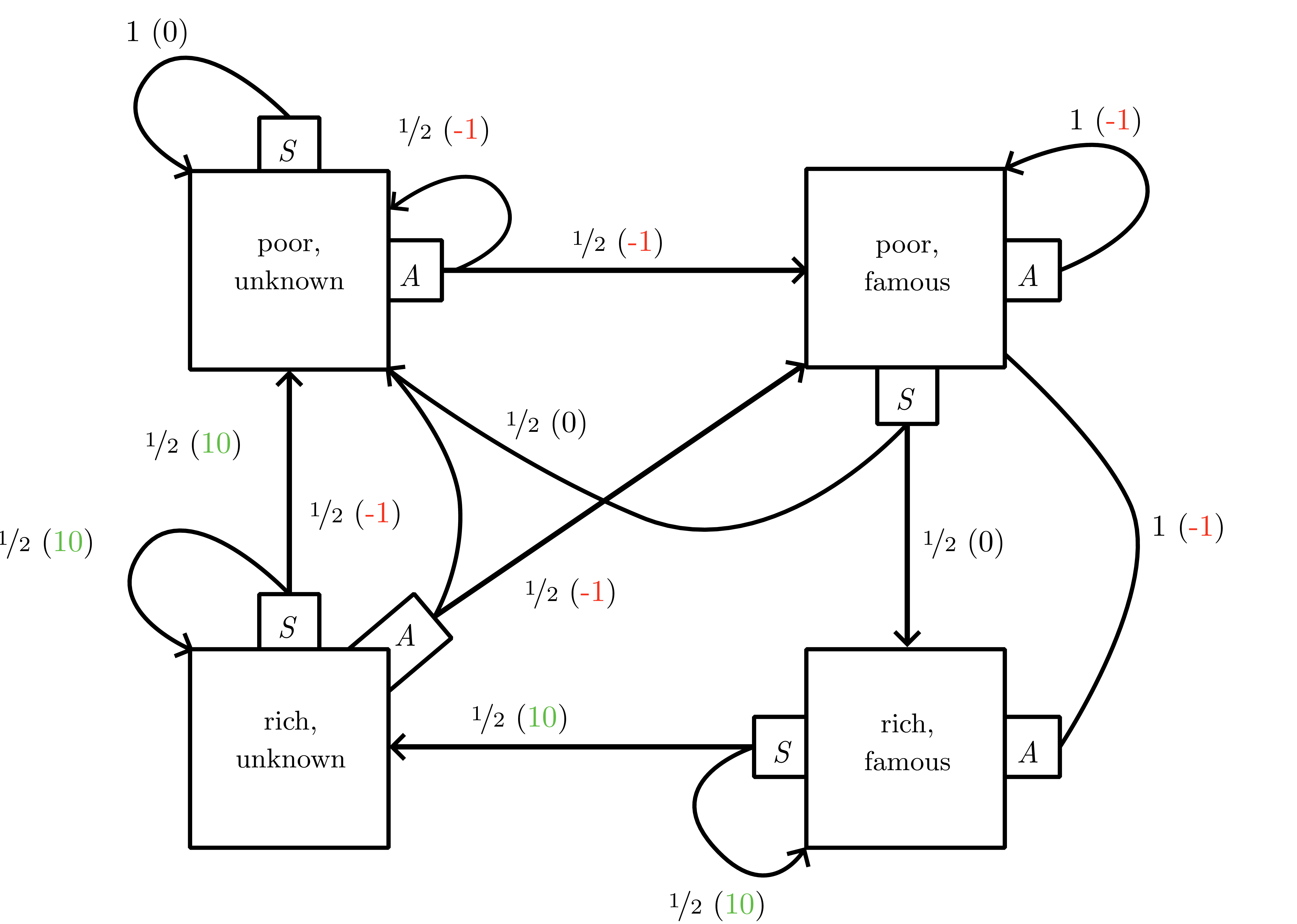 {#fig-10-mdp_example fig-align=“center” width=“80%”rich and famous” MDP: saving yields short-term reward but advertising unlocks future high-payoff states.”}
- Greedy wrt \(v\): \(\pi_v(x)=\arg\max_a r(x,a)+\gamma\sum_{x'}p(x'\mid x,a)v(x')\) (same as \(\arg\max_a q(x,a)\)).
- Policy improvement theorem: \(v^{\pi_v}\ge v\); strict for some \(x\) unless \(v\equiv v^*\). Use this to define partial order over policies and establish existence of deterministic \(\pi^*\).
Exact solution algorithms
- Policy iteration (Alg. 10.1)
- Policy evaluation: solve \((I-\gamma P^{\pi_t}) v^{\pi_t} = r^{\pi_t}\) (direct solve \(\mathcal{O}(|\mathcal{X}|^3)\) or iterative).
- Improvement: \(\pi_{t+1}=\pi_{v^{\pi_t}}\).
- Monotone convergence (Lemma 10.7); terminates in finitely many steps because only finitely many deterministic policies exist. Linear convergence bound \(\|v^{\pi_t}-v^*\|_\infty\le\gamma^t\|v^{\pi_0}-v^*\|_\infty\).
- Linear programming formulation (Bellman inequalities) gives alternative derivation and underpins reward shaping (see
reward_modificationexercise).
- Value iteration (Alg. 10.2)
- Start with optimistic \(v_0(x)=\max_a r(x,a)\) (or zero) and iterate \(v_{t+1}=B^* v_t\).
- Converges to \(v^*\) asymptotically; \(\epsilon\)-optimal after \(\mathcal{O}(\log(\epsilon^{-1})/(1-\gamma))\) sweeps. Each sweep costs \(\mathcal{O}(|\mathcal{X}||\mathcal{A}|)\) if transitions sparse.
- Dynamic-programming interpretation: \(v_t\) = optimal return for \(t\)-step horizon + terminal reward \(0\).
- Asynchronous variants: Gauss-Seidel or prioritized sweeping still contract; practical for large tables.
POMDPs and belief MDPs
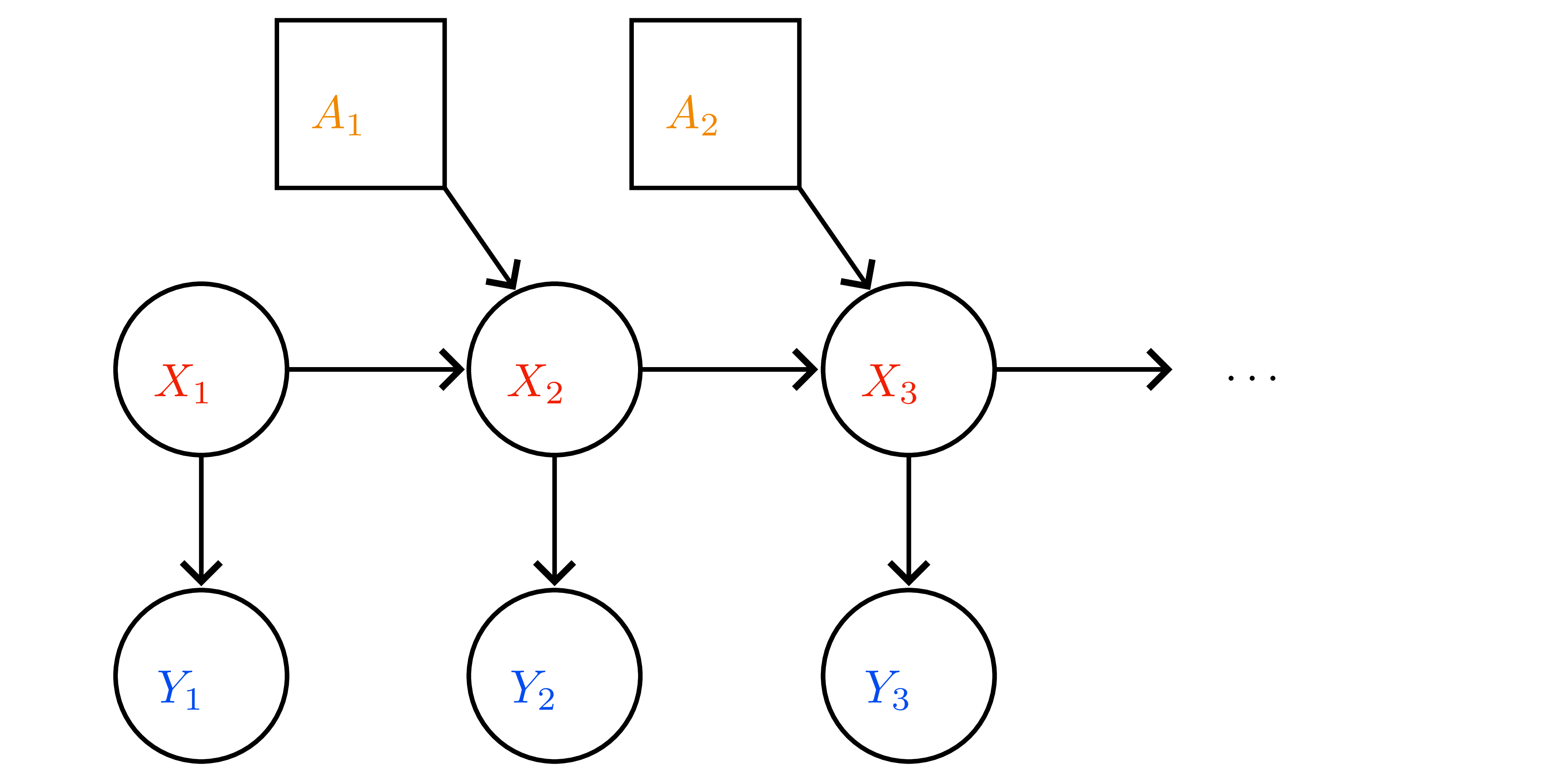
- POMDP \(=(\mathcal{X},\mathcal{A},\mathcal{Y},p,o,r)\); observation model \(o(y\mid x)\).
- Filtering update (Bayes):
- Predict: \(\bar{b}_{t+1}(x)=\sum_{x'}p(x\mid x',a_t)b_t(x')\).
- Update: \(b_{t+1}(x)=\frac{o(y_{t+1}\mid x)\bar{b}_{t+1}(x)}{\sum_{x''}o(y_{t+1}\mid x'')\bar{b}_{t+1}(x'')}\).
- Belief MDP: state space is simplex \(\Delta^{\mathcal{X}}\), reward \(\rho(b,a)=\sum_x b(x)r(x,a)\), transition kernel \(\tau(b'\mid b,a)=\sum_{y} \mathbf{1}\{b' = \text{BeliefUpdate}(b,a,y)\} \Pr(y\mid b,a)\).
- Exact planning infeasible (continuous state). Motivates approximate solvers (point-based value iteration, particle filters) later; Kalman filtering handles the linear-Gaussian case.
Safety, reward shaping, and convergence notes
- Reward scaling (\(r' = \alpha r\)) leaves optimal policy invariant; additive constants may change optimal policy (exercise
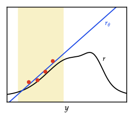
reward_modification). Potential-based shaping \(f(x,x')=\gamma\phi(x')-\phi(x)\) preserves optimal policies and avoids clever gamers exploiting hacked bonuses (see simulated “reward gaming” below).
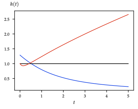
- Mixing-time perspective: fundamental theorem of ergodic Markov chains (see ?@fig-06-mc_examples ) ensures convergence of state distribution under stationary policy; visualize waiting times to revisit states via the coupon-collector-style decay below.
Cross-links for later chapters
- Discounted payoff definition reused in all subsequent RL chapters.
- Greedy-with-respect-to-value operator \(\pi_v\) reappears in policy iteration style updates for both tabular and approximate RL.
- Belief-state construction is the conceptual bridge to latent world models and particle filtering in model-based RL.