Bayesian Optimization
Overview
Black-box optimization with a probabilistic surrogate (typically a Gaussian process). Balances exploration vs exploitation via acquisition functions while connecting to bandit intuition and RL planning.
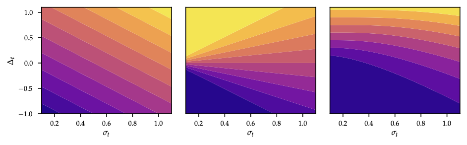
As shown in Figure 1, PI, EI, and UCB respectively focus exploitation vs exploration for a 2D Branin-like surface.
Problem setup
- Unknown objective \(f:\mathcal{X}\to\mathbb{R}\); observations \(y_t = f(x_t) + \varepsilon_t\), \(\varepsilon_t\sim\mathcal{N}(0,\sigma_n^2)\).
- Surrogate: GP posterior \((\mu_t(x),\sigma_t^2(x))\) after \(t\) queries.
- Acquisition \(a_t(x)\) selects next query \(x_{t+1}=\arg\max_x a_t(x)\).
- Trade-off: exploration (high \(\sigma_t\)) vs exploitation (high \(\mu_t\)).
Upper Confidence Bound (UCB)
- Optimism in face of uncertainty (OFU): \[x_{t+1}=\arg\max_x \mu_t(x)+\beta_{t+1}^{1/2}\,\sigma_t(x).\]
- \(\beta_t\) controls confidence width; choose schedule to guarantee \(f(x)\in[\mu_t(x)\pm\beta_t^{1/2}\sigma_t(x)]\) with high prob.
- Bayesian setting: \(\beta_t = 2\log\frac{|\mathcal{X}|\pi^2 t^2}{6\delta}\) (finite domain). Frequentist: \(\beta_t= B + 4\sigma_n\sqrt{\gamma_{t-1}+1+\ln(1/\delta)}\) when \(f\) bounded in RKHS (Theorem 9.3).
- Regret bound \(\mathcal{O}(\sqrt{T\beta_T\gamma_T})\) where \(\gamma_T\) is information gain of kernel (RBF: \(\gamma_T=\tilde{\mathcal{O}}((\log T)^{d+1})\)).
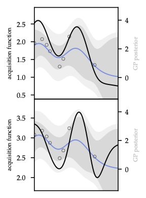
As Figure 2 illustrates, confidence tubes widen on sparse data, making the optimism term explicit.
Improvement-based acquisition
- Maintain incumbent best \(\hat{f}_t=\max_{\tau\le t} y_\tau\).
- Probability of improvement (PI): \[a_t^{\mathrm{PI}}(x)=\Phi\Big(\frac{\mu_t(x)-\hat{f}_t-\xi}{\sigma_t(x)}\Big)\] with exploration parameter \(\xi\ge0\) (larger \(\xi\) encourages exploration).
- Expected improvement (EI): \[a_t^{\mathrm{EI}}(x) = (\mu_t(x)-\hat{f}_t-\xi)\Phi(z) + \sigma_t(x)\phi(z),\quad z=\frac{\mu_t(x)-\hat{f}_t-\xi}{\sigma_t(x)}.\] Closed form for Gaussian surrogate; often optimize \(\log\text{EI}\) to avoid flatness.
- Both rely on Gaussian predictive distribution; for non-Gaussian surrogates use quadrature or MC.
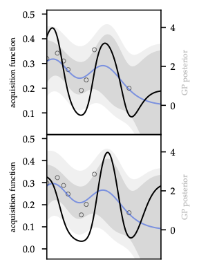
As Figure 3 shows, PI saturates once \(\mu_t\) exceeds the incumbent, whereas EI still values high-variance points — the ridge over \(\hat{f}_t\) remains.
Thompson sampling / probability matching
- Sample function \(\tilde{f}\sim\mathcal{GP}(\mu_t,k_t)\) and pick \(x_{t+1}=\arg\max_x \tilde{f}(x)\).
- Equivalent to sampling from probability of optimality distribution \(\pi(x)=\Pr[\tilde{f}(x)=\max_x \tilde{f}(x)]\).
- Implement via random Fourier features or basis projection to draw approximate GP sample.
Exploratory design connections
- MI view: \(\Delta_I(x)=\tfrac{1}{2}\log(1+\sigma_t^{-2}(x)\sigma^2_{\varepsilon})\) for GP ⇒ UCB/EI can be seen as MI proxies.
- Knowledge gradient / information-directed sampling combine expected reward improvement with information gain.
- Acquisition trade-offs often tuned by schedule \(\beta_t\), \(\xi_t\), or entropy regularization.
Optimization of acquisition
- Non-convex; in low \(d\) use dense grids + local optimization, in higher \(d\) use multi-start gradient ascent, evolutionary strategies, or sample-evaluate heuristics.
- Warm-start new acquisition maximization from previous maximizers.
- Constraints: handle by penalizing infeasible points or modeling constraint GP.
Practicalities
- Hyperparameters: re-optimize GP kernel parameters via marginal likelihood after each few observations; rely on priors to avoid overfitting small data.
- Noise estimation: inaccurate noise variance breaks UCB/EI calibration.
- Batch BO: choose multiple points per round via fantasizing or \(q\)-EI/TS.
- Termination: when acquisition near zero or budget exhausted.
Links forward
- UCB-style optimism echoes exploration bonuses in RL.
- Thompson sampling in model space mirrors ensemble sampling strategies for world models.
- Entropy-based acquisition sets the stage for maximum-entropy RL.