Bayesian Deep Learning
Overview
Aim: extend Bayesian linear ideas to neural nets, quantify both epistemic/aleatoric uncertainty, and keep models calibrated. Techniques here fuel VI with neural nets, dropout-as-inference, ensembles, and RL exploration bonuses later.
From MAP to Bayesian neural nets
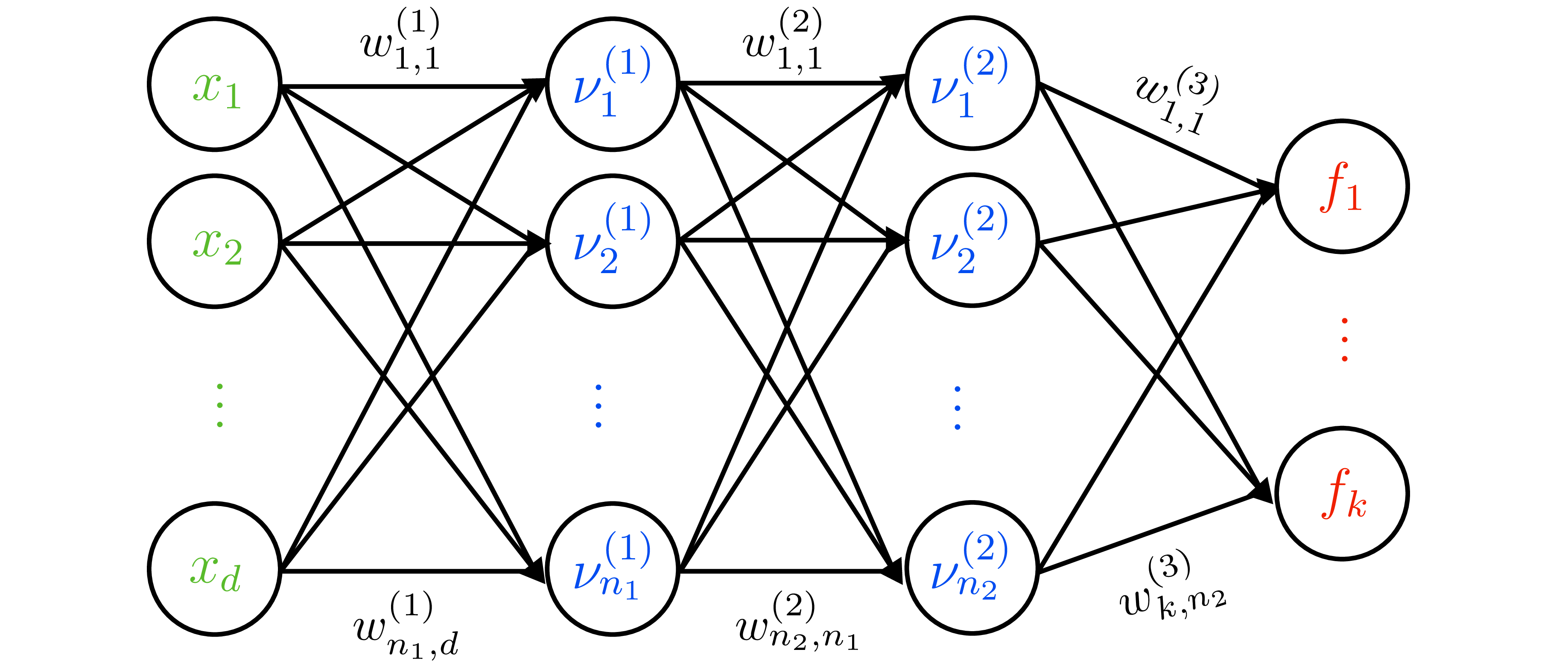
- Deterministic NN: \(f(x;\theta)=W_L\varphi(W_{L-1}\cdots\varphi(W_1 x))\).
- Likelihood for regression: \(y\mid x,\theta\sim\mathcal{N}(f(x;\theta),\sigma_n^2)\). MAP corresponds to weight decay (Gaussian prior \(\mathcal{N}(0,\sigma_p^2I)\)).
- Heteroscedastic likelihood: two-headed output \((\mu(x), \log\sigma^2(x))\) with \(y\mid x,\theta\sim\mathcal{N}(\mu(x),\sigma^2(x))\). Encourages model to learn input-dependent aleatoric noise.
Variational inference (Bayes by Backprop)
- Variational family: factorized Gaussian \(q_\lambda(\theta)=\prod_j \mathcal{N}(\mu_j,\sigma_j^2)\).
- ELBO: \[\mathcal{L}(\lambda)=\mathbb{E}_{q_\lambda}[\log p(\mathcal{D}\mid\theta)] - \operatorname{KL}(q_\lambda\|p(\theta)).\]
- Use reparameterization \(\theta=\mu+\sigma\odot\varepsilon\), \(\varepsilon\sim\mathcal{N}(0,I)\) to obtain low-variance gradients.
- Predictions: Monte Carlo average \(\tfrac{1}{M}\sum_{m}p(y^*\mid x^*,\theta^{(m)})\) with \(\theta^{(m)}\sim q_\lambda\).
- SWA/SWAG: collect SGD iterates \(\{\theta^{(t)}\}\), compute empirical mean/covariance, sample Gaussian weights at test time — cheap posterior approximation.
Dropout, dropconnect, masksembles
- Dropout: randomly zero activations; dropconnect: randomly zero weights. Gal & Ghahramani: interpret as variational posterior \(q_j(\theta_j)=p\,\delta_0+(1-p)\,\delta_{\lambda_j}\).
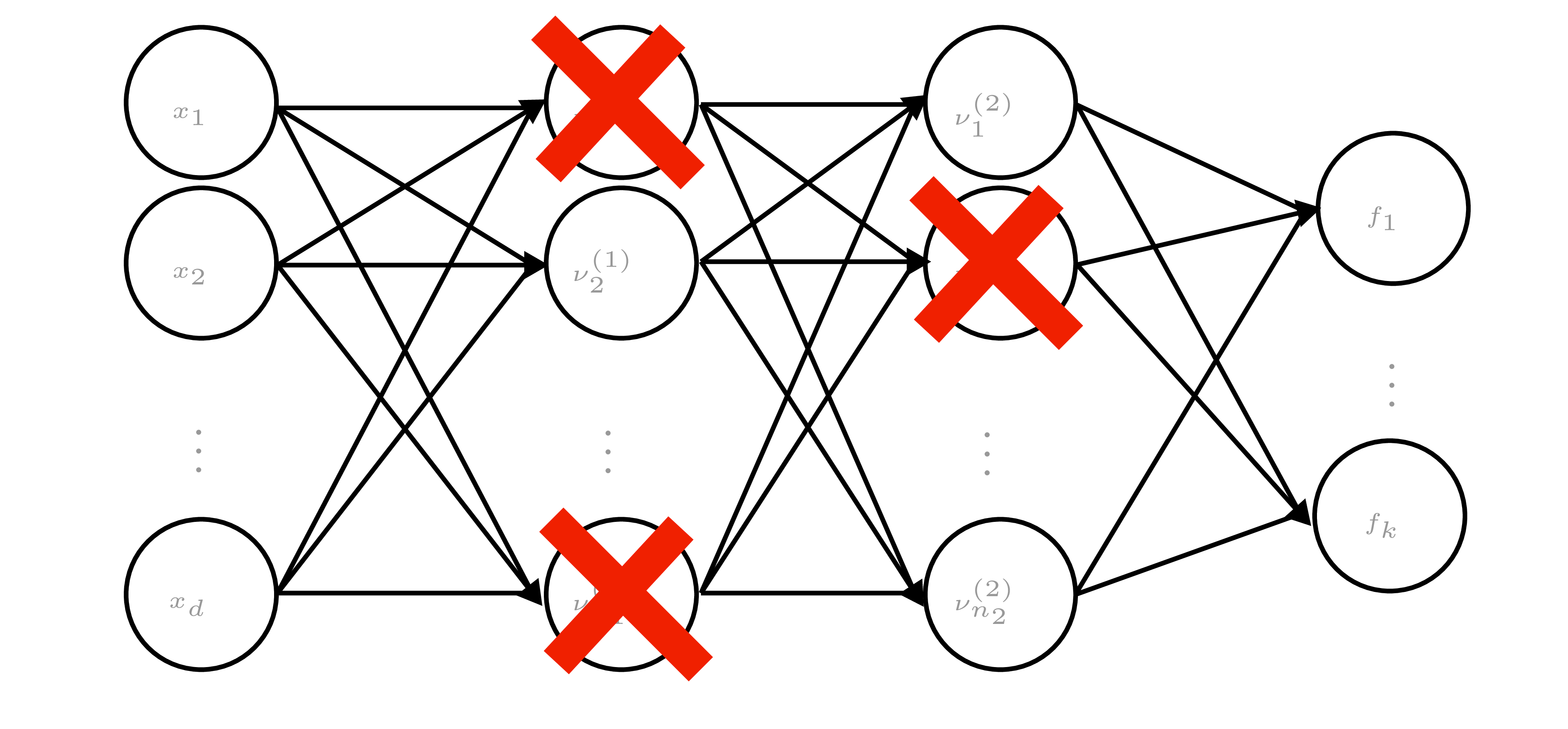
- Training objective (with weight decay) = ELBO for this \(q_j\). Prediction requires MC dropout (sample masks at test time to capture epistemic uncertainty).
- Masksembles: use fixed set of masks with controlled overlap to reduce correlation between subnets.
Probabilistic ensembles
- Train \(m\) models \(\{\theta^{(i)}\}\) (bootstrapped data or random init). Predictive distribution \(\approx\tfrac{1}{m}\sum_i p(y^*\mid x^*,\theta^{(i)})\).
- Mix with other approximations: e.g., each member uses SWAG or Laplace to yield mixture-of-Gaussians posterior.
- Empirical success in OOD detection, uncertainty calibration, and model-based RL.
Calibration diagnostics and fixes
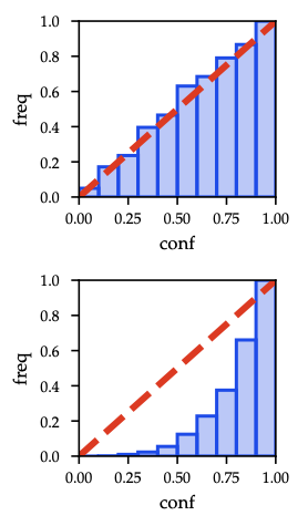
As shown in Figure 4, perfect calibration lies on the diagonal; shaded bars mark empirical accuracy gaps.
- A model is calibrated if predicted confidence matches empirical accuracy.
- Metrics: expected calibration error (ECE), maximum calibration error (MCE).
- Techniques:
- Histogram binning: map each confidence bin to empirical frequency.
- Isotonic regression: learn monotone piecewise-constant mapping.
- Platt scaling: fit sigmoid \(\sigma(a z + b)\) to logits.
- Temperature scaling (below): special case (\(b=0\)) adjusting sharpness without changing argmax.
- Evaluate on held-out validation set; essential when using uncertainty for decision-making (e.g., safe RL).
Key takeaways
- MAP yields point predictions only; capturing epistemic uncertainty requires VI, dropout-as-VI, SWAG, or ensembles.
- MC averaging at test time is non-negotiable when using stochastic approximations.
- Proper calibration is necessary before feeding uncertainties into downstream tasks (active learning, Bayesian optimization, safe RL).