Markov Chain Monte Carlo
Overview
Turn posterior sampling into Markov-chain design for cases where variational approximations fall short.

Markov-chain preliminaries
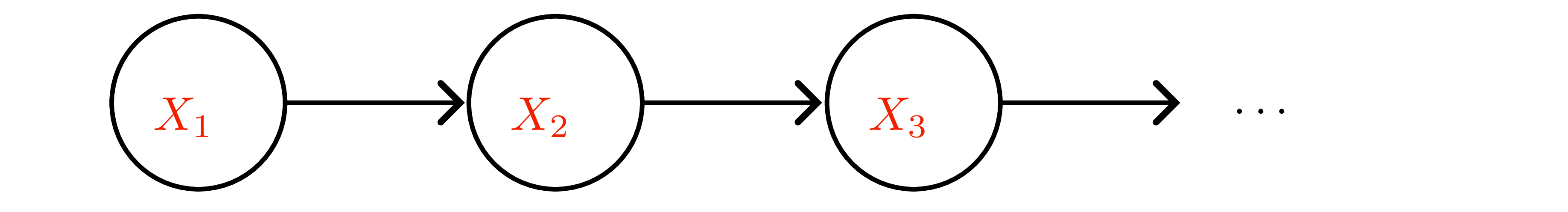
- Homogeneous chain with transition kernel \(P(x'\mid x)\); \(k\)-step transition \(P^k\).
- Stationary distribution \(\pi\) solves \(\pi^\top P = \pi^\top\). If chain is irreducible and aperiodic (ergodic), \(q_t\to\pi\) for any start (Fundamental theorem; see Figure 2 ).
- Detailed balance \(\pi(x)P(x'\mid x)=\pi(x')P(x\mid x')\) suffices for stationarity (reversibility).
- Distance to stationarity measured in total variation \(\|q_t-\pi\|_{\mathrm{TV}}\); mixing time \(\tau_{\mathrm{mix}}(\epsilon)\) ≈ steps to get within \(\epsilon\).
Metropolis–Hastings (MH)
- Goal: target density \(p(x)=q(x)/Z\) (unnormalized \(q\) known).
- Proposal \(r(x'\mid x)\); accept with \[\alpha(x'\mid x)=\min\left\{1,\frac{q(x')r(x\mid x')}{q(x)r(x'\mid x)}\right\}.\]
- Ensures detailed balance w.r.t. \(p\).
- Tuning: poor proposals ⇒ slow mixing (random walk). Adaptive schemes adjust step size to hit desired acceptance (≈0.234 in high-dims for isotropic random walk).
Gradient-informed proposals
- MALA: \(x' = x + \tfrac{\epsilon^2}{2}\nabla\log q(x) + \epsilon\xi\) (Langevin step) then MH accept; leverages gradient, useful in high dimension.
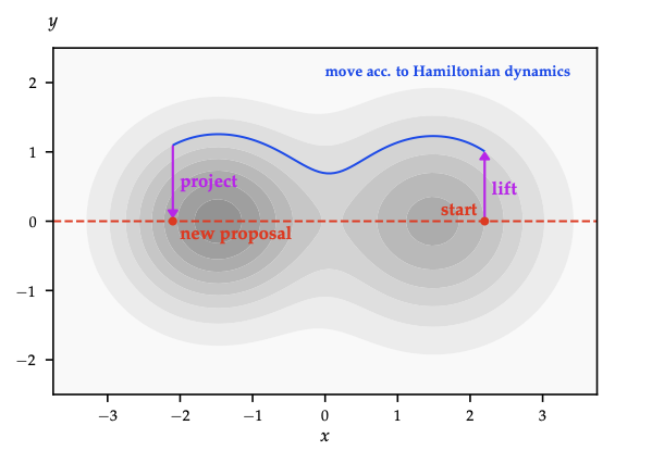
- HMC: introduce momentum \(p\sim\mathcal{N}(0,M)\), simulate Hamiltonian dynamics, accept via MH. Long, low-rejection moves reduce random walk behaviour; requires gradient of \(\log q\).
- Riemannian manifold HMC: adapt metric to local curvature.
Gibbs sampling
- Cycle through coordinates (or blocks): sample \(x_i \sim p(x_i\mid x_{-i})\).
- Special case of MH with unit acceptance. Works when all conditionals easy; order can be fixed or random (random scan preserves detailed balance).
- Block Gibbs improves mixing when variables correlated.
Practical workflow
- Initialize (multiple chains if possible).
- Burn-in until diagnostics (trace plots, potential scale reduction \(\hat{R}\)) stabilize.
- Collect samples, optionally thin to reduce storage (does not improve ESS).
- Estimate expectations via Monte Carlo averages; report Monte Carlo error using ESS or batch means.
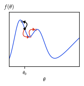
Energy interpretation
- Target \(p(x) \propto e^{-E(x)}\) with energy \(E(x)=-\log q(x)\).
- Random-walk MH explores energy landscape slowly; Langevin/HMC follow gradient/level sets ⇒ faster exploration.
- Simulated tempering / parallel tempering mix chains at different temperatures to escape local modes.
When to choose MCMC
- High-fidelity posterior samples needed (e.g., small models with multimodality) and gradient evaluations affordable.
- Combine with VI: use VI for initialization, then MCMC for refinement (e.g., Laplace+MCMC).
- Expensive in high dimension; mixing diagnostics essential.
MCMC keeps normalization outside the loop; designing good proposals is the art. Understanding irreducibility, acceptance ratios, and diagnostics is crucial before scaling to Bayesian deep learning or world-model uncertainty.