Variational Inference
Overview
Approximate Bayesian inference by optimization. Provides the ELBO machinery that powers probabilistic deep learning, RL, and latent world models.
From Laplace to VI
- Laplace: second-order Taylor of log-posterior around MAP \(\hat{\theta}\) ⇒ Gaussian \(q(\theta)=\mathcal{N}(\hat{\theta},(-\nabla^2\log p)^{-1})\). Good for unimodal, local approximations; ignores skew/tails.
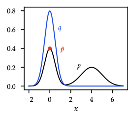
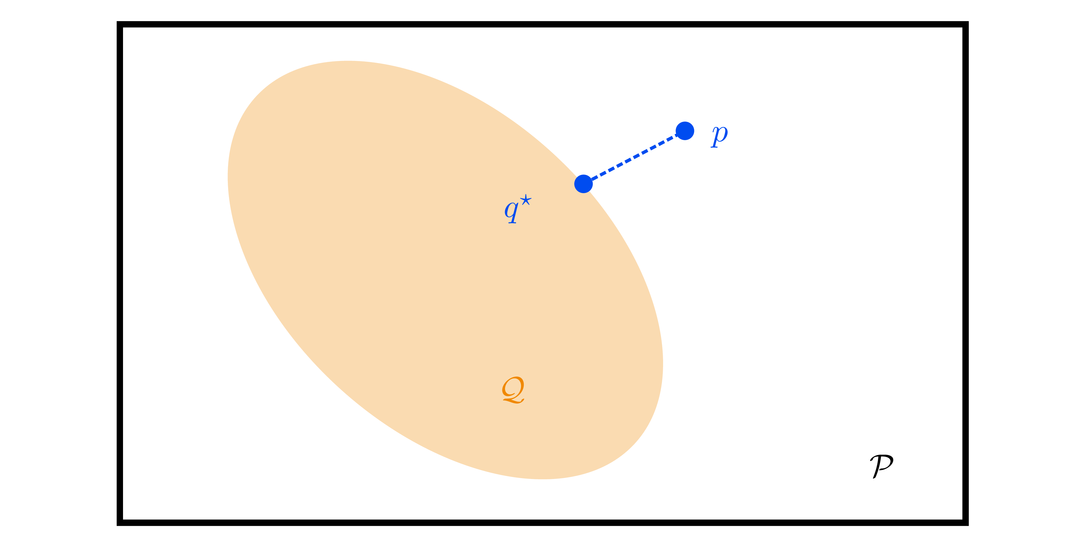
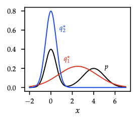
- Variational inference generalizes: choose family \(\mathcal{Q}=\{q_{\lambda}(\theta)\}\), solve \[q^* = \arg\min_{q\in\mathcal{Q}} \mathrm{KL}(q\|p(\theta\mid\mathcal{D})).\] Reverse KL is mode-seeking (prefers concentrated approximations), complementing forward-KL moment-matching (EM-style) in exponential families.
ELBO identities
- Evidence lower bound (ELBO): \[\mathcal{L}(q)=\mathbb{E}_q[\log p(\mathcal{D},\theta)] + \mathcal{H}(q).\]
- Relationship: \(\log p(\mathcal{D}) = \mathcal{L}(q) + \mathrm{KL}(q\|p(\theta\mid\mathcal{D}))\) ⇒ maximizing ELBO minimizes reverse KL.
- Expanded: \(\mathcal{L}(q) = \mathbb{E}_q[\log p(\mathcal{D}\mid\theta)] - \mathrm{KL}(q\|p(\theta))\) — data fit vs regularization.
- Noninformative prior (\(p(\theta)\propto 1\)) ⇒ maximize average log-likelihood + entropy (maximum-entropy principle).
Gradient estimators
- Need \(\nabla_{\lambda} \mathcal{L}(q_{\lambda})\).
- Score-function estimator (REINFORCE): \[\nabla_{\lambda} \mathbb{E}_q[f(\theta)] = \mathbb{E}_q[f(\theta)\nabla_{\lambda}\log q_{\lambda}(\theta)],\] general but high variance ⇒ use baselines/control variates (Lemma 5.6).
- Reparameterization trick (Thm. 5.8): express \(\theta=g(\varepsilon;\lambda)\) with \(\varepsilon\sim p(\varepsilon)\) independent of \(\lambda\), then \[\nabla_{\lambda} \mathbb{E}_q[f(\theta)] = \mathbb{E}_{\varepsilon}[\nabla_{\lambda} f(g(\varepsilon;\lambda))].\] For Gaussian \(q_{\lambda}\): \(\theta=\mu+L\varepsilon\), \(\varepsilon\sim\mathcal{N}(0,I)\). Backbone of black-box VI, VAEs, and policy gradients with reparameterized actions.
Practical VI recipe
- Choose family \(q_{\lambda}(\theta)\) (mean-field Gaussian, full-covariance, normalizing flows, etc.).
- Write ELBO; split analytic terms (KL for Gaussians) vs MC terms (expected log-likelihood).
- Estimate gradients using reparameterization or score-function + baselines.
- Optimize with SGD/Adam; optionally natural gradients (mirror descent under KL geometry).
Predictive inference
- Approximate predictive \(p(y^*\mid x^*,\mathcal{D}) \approx \int p(y^*\mid x^*,\theta)q(\theta)d\theta\) via Monte Carlo.
- For GLM with Gaussian \(q\): integrate out weights analytically to 1-D latent \(f^*\sim\mathcal{N}(\mu^\top x^*, x^{*\top}\Sigma x^*)\), then compute \(\int p(y^*\mid f^*)\mathcal{N}\) (e.g., logistic regression uses Gauss-Hermite quadrature or probit approximation).
Information-theoretic view
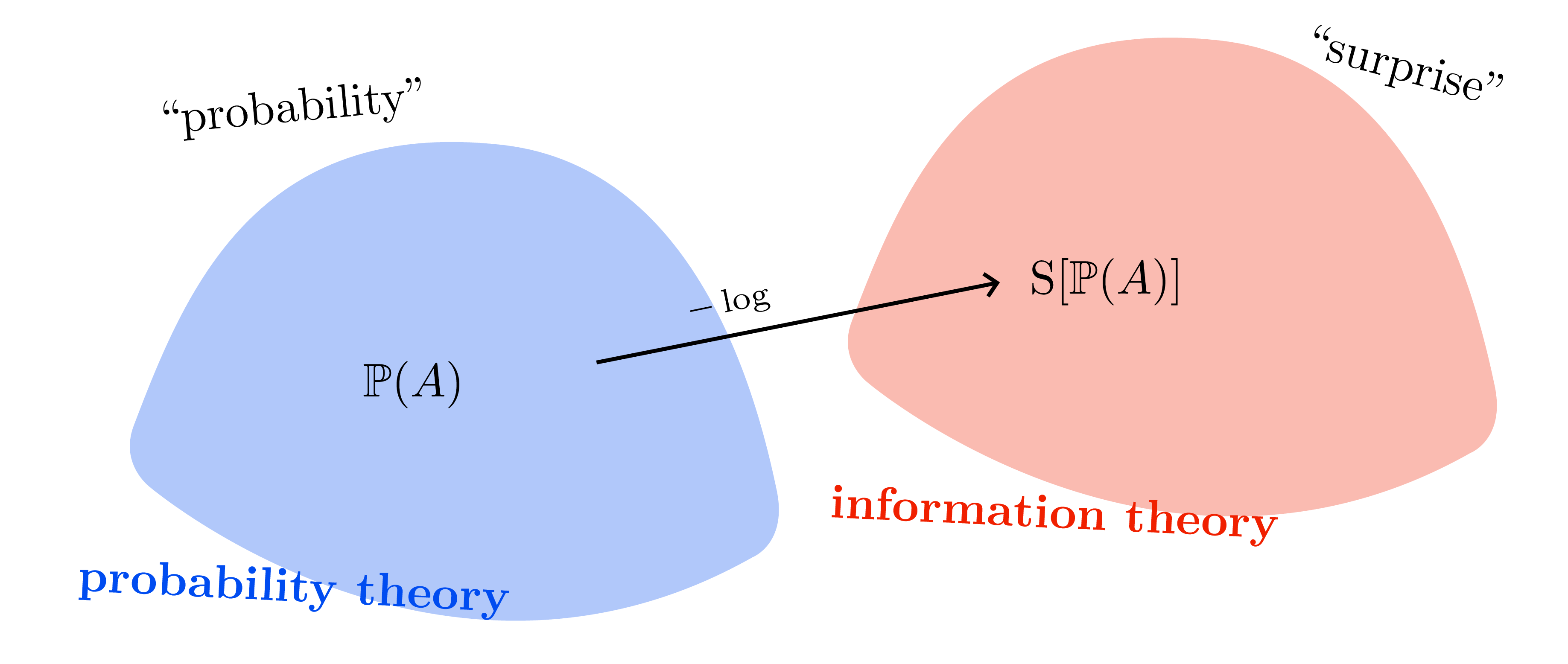
- Free energy \(F(q)=-\mathcal{L}(q)=\mathbb{E}_q[\mathcal{S}(p(\mathcal{D},\theta))] - \mathcal{H}(q)\).
- Minimizing \(F\) trades “energy” (data fit) against entropy (spread). The same curiosity vs conformity principle shows up in max-entropy RL and exploration bonuses.
Choice of variational family
- Mean-field Gaussian ⇒ two parameters per latent; cheap but ignores correlations (underestimates variance).
- Full-covariance Gaussian ⇒ \(\mathcal{O}(d^2)\) params.
- Structured families: mixture of Gaussians, low-rank plus diagonal, normalizing flows (invertible transforms) for richer posterior shapes.
- Hierarchical priors/hyperpriors: introduce latent hyperparameters \(\eta\), augment \(q(\theta,\eta)\) with factorization.
Connections to later chapters
- Score-function estimator = REINFORCE gradient with baselines derived here.
- Reparameterization trick reappears in stochastic value gradients and dropout-as-VI.
- Free-energy viewpoint parallels entropy-regularized RL and active-learning acquisition design.