Bayesian Filtering

Overview

Sequential inference over hidden states. Kalman filtering is the linear-Gaussian case; smoothing/prediction variants reappear in downstream planning settings.

Figure 1: Bayesian filtering: perceive the world state and update the latent belief.

Linear-Gaussian state-space model

Latent state \(x_t\in\mathbb{R}^d\), observation \(y_t\in\mathbb{R}^m\).
Dynamics (motion) \(x_{t+1}=Fx_t+\varepsilon_t\), \(\varepsilon_t\sim\mathcal{N}(0,\Sigma_x)\).
Observation (sensor) \(y_t=Hx_t+\eta_t\), \(\eta_t\sim\mathcal{N}(0,\Sigma_y)\).
Prior \(x_0\sim\mathcal{N}(\mu_0,\Sigma_0)\); noises independent.
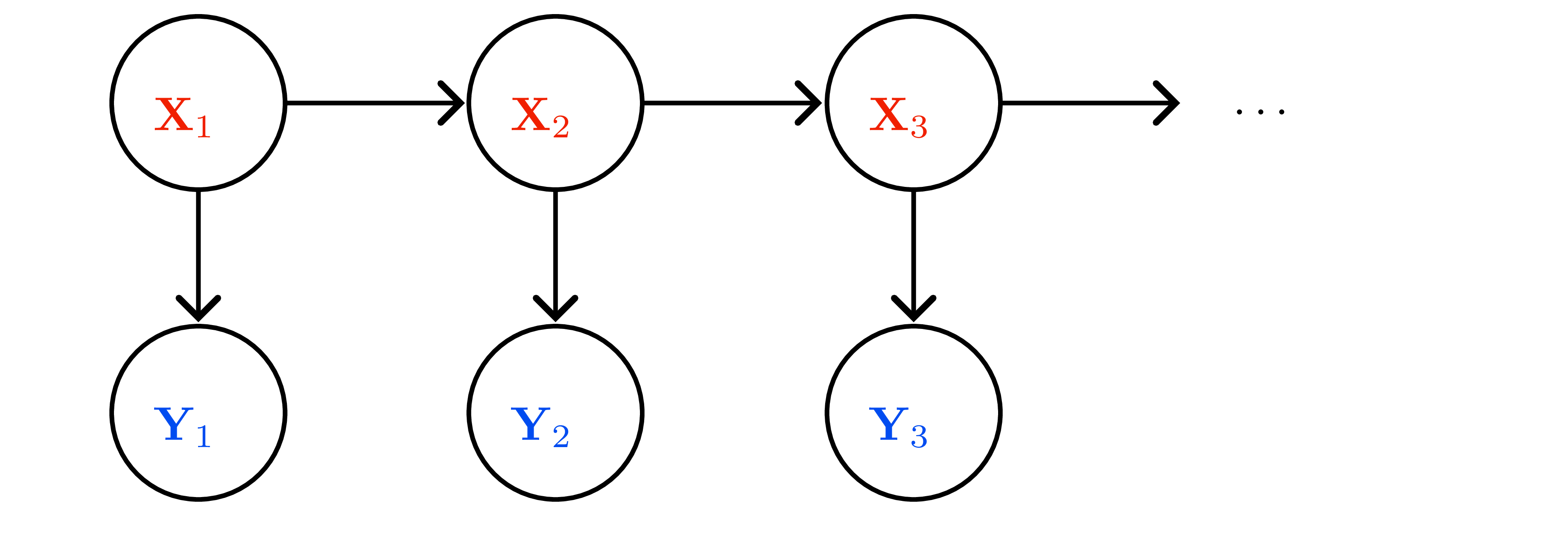
Graphical model (Figure 2): Markov property \(x_{t+1}\perp x_{0:t-1},y_{0:t-1}\mid x_t\); measurement independence \(y_t\perp x_{0:t-1},y_{0:t-1}\mid x_t\).

Figure 2: Graphical model of a Kalman filter with hidden states \(X_t\) and observations \(Y_t\).

Kalman filter recursion

Belief \(p(x_t\mid y_{1:t}) = \mathcal{N}(\mu_t,\Sigma_t)\).

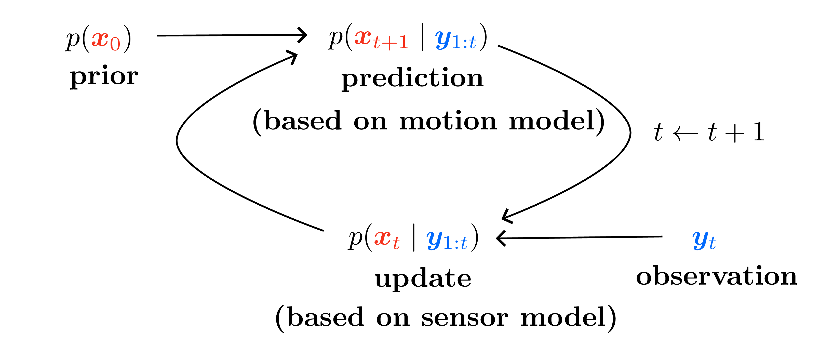
Predict (time update) \[\hat{\mu}_{t+1}=F\mu_t,\qquad \hat{\Sigma}_{t+1}=F\Sigma_t F^\top + \Sigma_x.\]
Update (measurement)
- Kalman gain \(K_{t+1}=\hat{\Sigma}_{t+1}H^\top(H\hat{\Sigma}_{t+1}H^\top+\Sigma_y)^{-1}\).
- Posterior mean/covariance: \[ \mu_{t+1}=\hat{\mu}_{t+1}+K_{t+1}(y_{t+1}-H\hat{\mu}_{t+1}),\quad \Sigma_{t+1}=(I-K_{t+1}H)\hat{\Sigma}_{t+1}. \]

Innovation \(y_{t+1}-H\hat{\mu}_{t+1}\) measures sensor surprise; \(K_{t+1}\) balances trust between prediction and measurement.

Scalar intuition

Random walk + noisy sensor: \(x_{t+1}=x_t+\varepsilon_t\), \(y_{t+1}=x_{t+1}+\eta_{t+1}\) with variances \(\sigma_x^2,\sigma_y^2\).
Posterior variance update \(\sigma_{t+1}^2=(1-\lambda)(\sigma_t^2+\sigma_x^2)\) where \[\lambda=\frac{\sigma_t^2+\sigma_x^2}{\sigma_t^2+\sigma_x^2+\sigma_y^2}.\]
\(\sigma_y^2\to0\) ⇒ trust measurements; \(\sigma_y^2\to\infty\) ⇒ ignore measurements.

Figure 3: Hidden states tracked during a one-dimensional random walk example.

Smoothing, prediction, control

Prediction: output \(\mathcal{N}(\hat{\mu}_{t+1},\hat{\Sigma}_{t+1})\) (no measurement).
Filtering: recursion above.
Smoothing: backward pass (Rauch–Tung–Striebel) refines past states once future measurements available — key in EM for LDS.
These three modes generalize to nonlinear filters (EKF/UKF) and particle filters when Gaussian assumptions fail.

Link to Bayesian linear regression

Treat weights \(w\) as static hidden state: \(F=I\), \(\Sigma_x=0\), \(H_t=\mathbf{x}_t^\top\), measurement \(y_t\) ⇒ Kalman filter updates reduce to sequential Bayesian linear regression.
Kalman gain matches recursive least squares gain.

Practical remarks

Time-invariant \((F,H,\Sigma_x,\Sigma_y)\) ⇒ \(K_t\) converges; can precompute steady-state solution via Riccati equation.
Initialization: choose \((\mu_0,\Sigma_0)\) to encode prior belief; large \(\Sigma_0\) yields “cold start” with aggressive measurement uptake.
Failure modes: unmodeled dynamics, non-Gaussian noise ⇒ need EKF/UKF, particle filters, or learned process models.

This chapter’s algebra (matrix Riccati, innovation form) underpins belief updates in POMDPs and latent world models alike.