Bayesian Linear Regression
Overview
First Bayesian workhorse: converts linear regression into a full posterior. Sets up the probabilistic tools reused by later chapters.

Linear-Gaussian model recap
- Data: inputs \(\mathbf{X}\in\mathbb{R}^{n\times d}\), labels \(\mathbf{y}\in\mathbb{R}^n\).
- Likelihood \(p(\mathbf{y}\mid\mathbf{w})=\prod_{i=1}^n \mathcal{N}(y_i\mid\mathbf{x}_i^\top\mathbf{w},\sigma_n^2)\) — Gaussian noise \(\varepsilon_i\sim\mathcal{N}(0,\sigma_n^2)\).
- Prior \(\mathbf{w}\sim\mathcal{N}(0,\sigma_p^2 I)\) ⇒ conjugate; ridge/MAP arises when replacing posterior with its mode.
- Posterior (complete the square): \[ \Sigma = (\sigma_n^{-2}\mathbf{X}^\top\mathbf{X} + \sigma_p^{-2}I)^{-1},\quad \mu = \sigma_n^{-2}\Sigma\mathbf{X}^\top\mathbf{y},\quad p(\mathbf{w}\mid\mathcal{D})=\mathcal{N}(\mu,\Sigma). \]
- Posterior collapses to MLE as \(\sigma_p^2\to\infty\); to prior as \(n\to0\).
Predictive distribution & variance decomposition
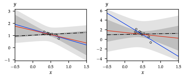
- Latent function \(f^* = \mathbf{x}_*^\top\mathbf{w}\) yields \(f^*\mid\mathcal{D},\mathbf{x}_*\sim\mathcal{N}(\mathbf{x}_*^\top\mu,\mathbf{x}_*^\top\Sigma\mathbf{x}_*)\).
- Observed target \(y^*\mid\mathcal{D},\mathbf{x}_*\sim\mathcal{N}(\mathbf{x}_*^\top\mu,\mathbf{x}_*^\top\Sigma\mathbf{x}_* + \sigma_n^2)\).
- Using law of total variance, predictive variance splits into epistemic \(\mathbf{x}_*^\top\Sigma\mathbf{x}_*\) (shrinks with data) + aleatoric \(\sigma_n^2\) (irreducible noise).
Online / Kalman-style updates
- Start with \((\mu^{(0)},\Sigma^{(0)})=(0,\sigma_p^2 I)\).
- Assimilate \((\mathbf{x}_t,y_t)\) via gain \(k_t = \frac{\Sigma^{(t-1)}\mathbf{x}_t}{\sigma_n^2+\mathbf{x}_t^\top\Sigma^{(t-1)}\mathbf{x}_t}\): \[ \mu^{(t)} = \mu^{(t-1)} + k_t(y_t - \mathbf{x}_t^\top\mu^{(t-1)}),\quad \Sigma^{(t)} = \Sigma^{(t-1)} - k_t\mathbf{x}_t^\top\Sigma^{(t-1)}. \]
- Identical algebra to Kalman filtering with a static state; cost \(\mathcal{O}(d^2)\) per update.
Function-space view and kernels
- Transform features with \(\boldsymbol{\phi}(x)\) (possibly infinite). Weight prior induces function prior: \[ f\mid\mathbf{X} \sim \mathcal{N}(0,\mathbf{K}),\quad K_{ij}=\sigma_p^2\,\boldsymbol{\phi}(\mathbf{x}_i)^\top\boldsymbol{\phi}(\mathbf{x}_j) = k(\mathbf{x}_i,\mathbf{x}_j). \]
- Predictive mean \(\mu'(x)=k(x,\mathbf{X})^{\top}(\mathbf{K}+\sigma_n^2 I)^{-1}\mathbf{y}\), predictive variance \(k'(x,x)=k(x,x)-k(x,\mathbf{X})^{\top}(\mathbf{K}+\sigma_n^2 I)^{-1}k(x,\mathbf{X})\).
- Removes need to explicitly materialize high-dimensional \(\boldsymbol{\phi}\) — the kernel trick in action.
Evidence maximization / empirical Bayes
- Marginal likelihood (evidence) of labels: \[ \log p(\mathbf{y}\mid\mathbf{X},\theta) = -\tfrac{1}{2}\mathbf{y}^\top\mathcal{C}^{-1}\mathbf{y} - \tfrac{1}{2}\log|\mathcal{C}| - \tfrac{n}{2}\log 2\pi, \] where \(\mathcal{C}=\sigma_n^2 I + \sigma_p^2 \mathbf{X}\mathbf{X}^\top\) and \(\theta=(\sigma_n,\sigma_p)\).
- Maximizing evidence trades fit term \(\mathbf{y}^\top\mathcal{C}^{-1}\mathbf{y}\) vs complexity term \(\log|\mathcal{C}|\); useful for hyperparameter tuning across Bayesian models.
Design choices & links forward
- Regularization perspective: prior variance \(\sigma_p^2\) controls weight shrinkage (ridge); different priors (Laplace, hierarchical) lead to sparse or hierarchical BLR.
- Posterior covariance \(\Sigma\) is the raw material for Thompson sampling, Bayesian optimization, and epistemic bonuses in model-based RL.
- Function-space formulation + evidence maximization form the blueprint for Gaussian processes, variational inference, and dropout-as-variational inference.