9 - Permutation Tests

A permutation test, also known as a randomization test, is a non-parametric statistical test used to determine if there is a significant difference between two or more groups. Unlike the bootstrap method, which involves resampling with replacement, permutation tests involve resampling without replacement.

Hypotheses in Permutation Tests

Permutation tests are often used to test the null hypothesis \(H_0\) that two distributions, \(f\) and \(g\), are identical, against the alternative hypothesis \(H_1\) that they are different.

• Null Hypothesis (\(H_0\)): \(f = g\)
• Alternative Hypothesis (\(H_1\)): \(f \neq g\)

They are called non-parametric because they do not assume any specific distribution of the data.

Methodology

1. Data Setup: Assume we have two groups of data:

   • \(x_1, x_2, \ldots, x_n\) from distribution \(f\)
   • \(y_1, y_2, \ldots, y_m\) from distribution \(g\)

   Define the combined ordered set \(z = (x_1, x_2, \ldots, x_n, y_1, y_2, \ldots, y_m)\) with \(N = n + m\).

2. Permutations: Let \(\pi_i\) denote a permutation that samples \(n\) elements from \(N\) without replacement. There are \(\binom{N}{n}\) possible permutations.

   Each permutation \(Z_{\pi_i}\) rearranges \(Z\) such that the first \(n\) elements are considered as group \(x\) and the remaining \(m\) elements as group \(y\).

3. Test Statistic: Define a test statistic \(\hat{\theta}(Z)\) based on the observed data. For example, if comparing means, it could be:

   \[ \hat{\theta} = \bar{Y}_B - \bar{X}_A \]

   where \(\bar{Y}_B\) and \(\bar{X}_A\) are the sample means of the two groups.

   For each permutation \(Z_{\pi_i}\), compute the statistic \(\hat{\theta}(Z_{\pi_i})\). This creates a permutation distribution of the test statistic.

Example: Testing Means

Consider two observations from groups A and B:

• Group A: \(3, 4\)
• Group B: \(5, 6\)

We want to test if the two groups have the same mean at the 0.05 significance level.

• Null Hypothesis (\(H_0\)): \(\mu_A = \mu_B\)

• Observed Data: \[ \bar{X}_A = 3.5, \quad \bar{Y}_B = 5.5 \] \[ \hat{\theta} = \bar{Y}_B - \bar{X}_A = 5.5 - 3.5 = 2 \]

  We calculate the test statistic for different permutations:

Permutation	Group A	Group B	\(\hat{\theta}(Z_{\pi_i})\)
(3, 4) (5, 6)	3, 4	5, 6	5.5 - 3.5 = 2
(3, 5) (4, 6)	3, 5	4, 6	5 - 4 = 1
(3, 6) (4, 5)	3, 6	4, 5	4.5 - 4.5 = 0
(4, 5) (3, 6)	4, 5	3, 6	4.5 - 4.5 = 0
(4, 6) (3, 5)	4, 6	3, 5	4 - 5 = -1
(5, 6) (3, 4)	5, 6	3, 4	3.5 - 5.5 = -2

Under \(H_0\), all permutations are equally likely. The test statistic values are discrete and uniformly distributed.

• Permutation Values: -2, -1, 0, 1, 2
• Probabilities: \(\frac{1}{6}\) for -2, -1, 1, 2, and \(\frac{1}{3}\) for 0.

The p-value is calculated as:

\[ P(\hat{\theta}(Z_{\pi_i}) \geq 2 \text{ or } \hat{\theta}(Z_{\pi_i}) \leq -2) = \frac{2}{6} = \frac{1}{3} \]

Since the p-value \(\frac{1}{3}\) is greater than 0.05, we do not reject \(H_0\).

Exact and Approximate Tests

• Exact Test: Uses all \(\binom{N}{n}\) permutations. The p-value is the fraction of permutations where the test statistic is as extreme or more extreme than the observed value.

  \[ \text{ASL} = \frac{1}{\binom{N}{n}} \sum_{i=1}^{\binom{N}{n}} I(\hat{\theta}(Z_{\pi_i}) \geq \hat{\theta}(Z)) \]

• Approximate Test: When the number of permutations is too large, a random sample of permutations is used. The approximate p-value is:

  \[ \text{ASL} \approx \frac{1}{B} \sum_{i=1}^{B} I(\hat{\theta}(Z_{\pi_i}) \geq \hat{\theta}(Z)) \]

  where \(B\) is the number of random permutations sampled.

R Code Example

nreps <- 10000
x <- chickwts$weight[chickwts$feed == "meatmeal"]
y <- chickwts$weight[chickwts$feed == "sunflower"]
z <- c(x, y)
n1 <- length(x)
n2 <- length(y)
n <- n1 + n2
v <- 1:n
reps <- numeric(nreps)
observed <- t.test(x, y)$statistic

for (i in 1:nreps) {
    perm <- sample(v, size = n1, replace = FALSE)
    xperm <- z[perm]
    yperm <- z[-perm]
    reps[i] <- t.test(xperm, yperm)$statistic
}

hist(reps)
points(observed, 0, pch = 16, col = 2)

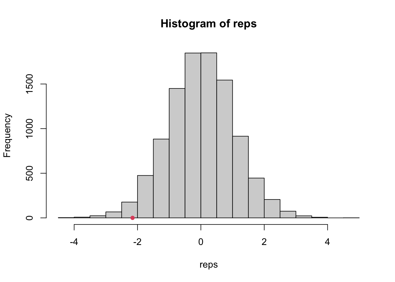
# Counting the number of times the replicates are more extreme than the observed
pval <- mean(abs(reps) > abs(observed))
pval

[1] 0.0417

observed_p <- t.test(x, y)$p.value
observed_p

[1] 0.04441462

Explanation: The code permutes the combined dataset, creates new datasets of the same size as the original groups, and calculates the t-statistic for each permutation. The p-value is the fraction of permutations where the test statistic is more extreme than the observed statistic. A low p-value indicates that the observed value is unlikely under the null hypothesis, leading us to reject \(H_0\).