x <- c(2, 2, 1, 1, 5, 4, 4, 3, 1, 2)
n <- length(x)
nboot <- 1000
theta_b <- numeric(nboot)
for (b in 1:nboot) {
    xb <- sample(x, n, replace = TRUE)
    theta_b[b] <- mean(xb)
}
hist(theta_b)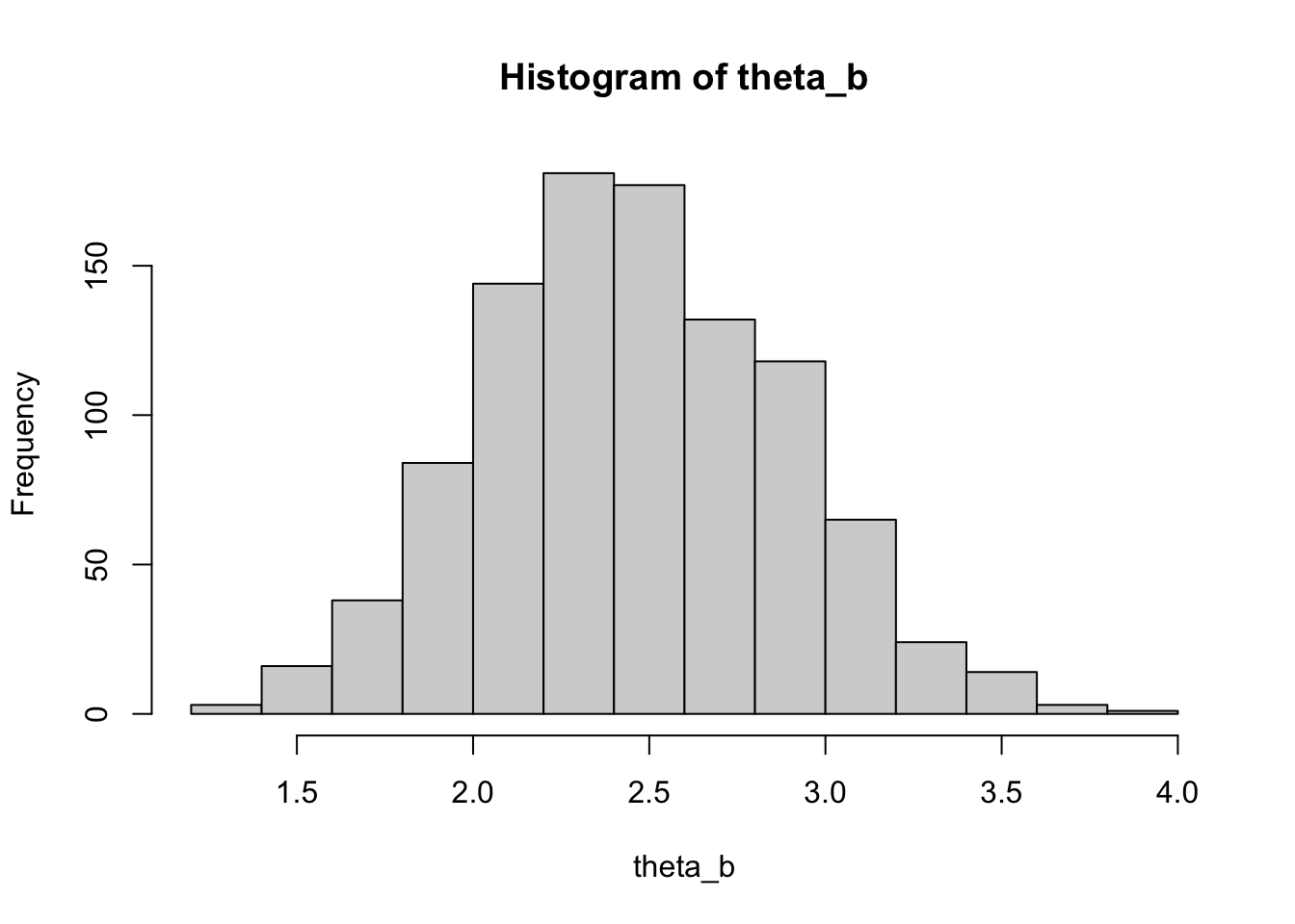
plot(density(theta_b))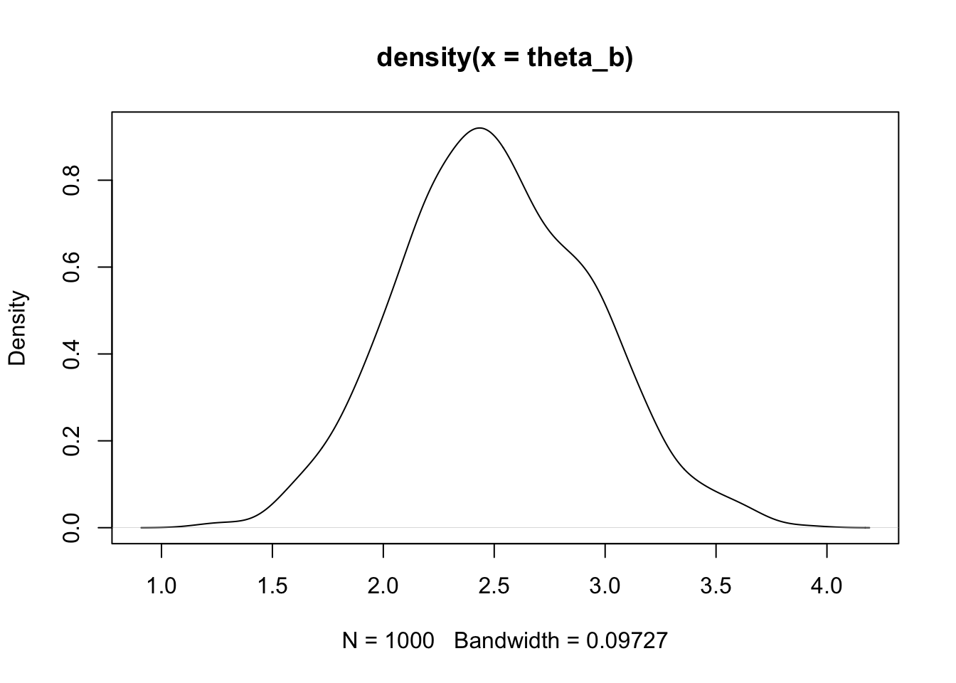
plot(ecdf(theta_b))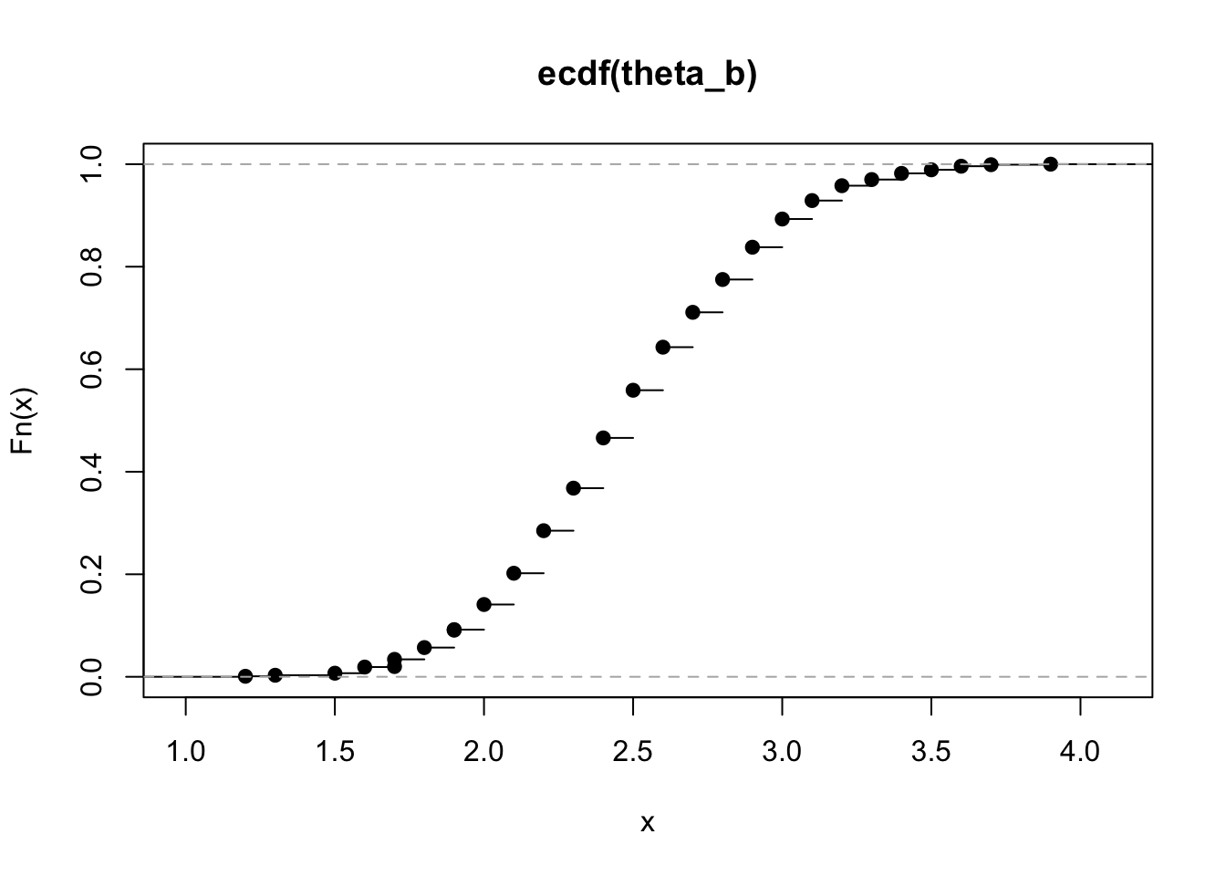
The Monte Carlo (MC) method based on resampling methods, as discussed in Chapter 7, is sometimes referred to as parametric bootstrap when simulating from a known distribution. We will now consider the nonparametric bootstrap.
Given \(n\) observations \(x_1, \ldots, x_n\), we don’t want to make any assumptions about the distribution. If the sample size is small, we cannot assume normality by the Central Limit Theorem (CLT).
Brad Efron introduced this method in 1979. Let \(x\) be a sample from \(F\), and let \(F_n\) be the empirical cumulative distribution function (CDF), defined as:
\[ F_n(x) = \frac{1}{n} \sum_{i=1}^n I(x_i \leq x) \]
\(F_n\) is an unbiased estimator of \(F\). We draw a random sample with replacement from the data:
sample(x, n, replace = TRUE)yielding a bootstrap sample \(x_b\). Alternatively, we can draw a random set of integers from \(1\) to \(n\).
Example: Estimating the distribution of the mean
x <- c(2, 2, 1, 1, 5, 4, 4, 3, 1, 2)
n <- length(x)
nboot <- 1000
theta_b <- numeric(nboot)
for (b in 1:nboot) {
xb <- sample(x, n, replace = TRUE)
theta_b[b] <- mean(xb)
}
hist(theta_b)
plot(density(theta_b))
plot(ecdf(theta_b))
Compute the mean, standard deviation, and quantiles of bootstrap replicates:
mean(theta_b)[1] 2.5081sd(theta_b)[1] 0.4302668quantile(theta_b, 0.5)50%
2.5 Using the law school dataset, we want to estimate the distribution of the correlation between LSAT and GPA:
library(bootstrap)
cor(law$LSAT, law$GPA)
[1] 0.7763745B <- 200
n <- nrow(law)
theta_b <- numeric(B)
for (b in 1:B) {
index <- sample(1:n, n, replace = TRUE)
theta_b[b] <- cor(law$LSAT[index], law$GPA[index])
}
hist(theta_b, prob = TRUE)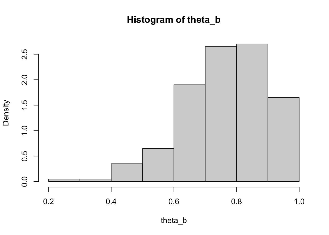
Bias \(\theta = E(\hat{\theta}) - \theta\)
Bias \(\hat{\theta} = \text{mean}(\hat{\theta}_b) - \hat{\theta}\)
This is the average of the bootstrap replicates minus the original estimate:
bias_theta_hat <- mean(theta_b) - cor(law$LSAT, law$GPA)
bias_theta_hat
[1] -0.01519128Discovered by Quenouille in 1949, the jackknife method involves leave-one-out cross-validation/resampling.
Given \(x = (x_1, x_2, \ldots, x_n)\):
Parameters are sometimes expressed as a function of the distribution \(\theta = \theta(F)\). For i.i.d. samples from \(F\):
If \(F_n\) is the EDF of \(x\), then an estimate of \(\theta\) can be expressed as \(\hat{\theta} = t(F_n)\).
An estimator is called smooth if it is a continuous function of the distribution function, meaning small changes in the data (hence \(F_n\)) correspond to small changes in the estimate. Population mean is tailored for normal and is smooth, whereas the median is not smooth.
The jackknife estimate of bias is:
\[ (n-1)(\text{mean}(\hat{\theta}_{(i)}) - \hat{\theta}) \]
The factor \((n-1)\) is included to correct for the bias of the bias estimate.
For a smooth estimator \(\theta\) of \(\hat{\theta}\):
\[ \text{SE} = \sqrt{\frac{n-1}{n} \sum(\hat{\theta}_{(i)} - \bar{\theta})^2} \]
where \(\bar{\theta} = \text{mean}(\hat{\theta}_{(i)})\).
When the jackknife fails: the estimator must be smooth.
Example: Median
n <- 10
x <- sample(1:100, n)
median_jack <- numeric(n)
for (i in 1:n) {
    median_jack[i] <- median(x[-i])
}
se <- sqrt((n - 1) / n * sum((median_jack - median(x))^2))
se
[1] 7.5The jackknife underestimates the standard error; the bootstrap estimate would be higher.
\(\hat{\theta} \pm z_{\alpha/2} \cdot \text{SE}_{\text{boot}}(\hat{\theta})\)
where \(\text{SE}_{\text{boot}}\) is the bootstrap estimate of the standard error calculated as the standard deviation of the bootstrap replicates:
\[ \text{SE}_{\text{boot}} = \sqrt{\frac{1}{B-1} \sum (\hat{\theta}_b - \text{mean}(\hat{\theta}))^2} \]
The intervals still rely on the asymptotic normality of the estimator.
Relaxes the normality assumption and uses quantiles of the bootstrap replicates, resulting in non-symmetric intervals:
\[ (2\hat{\theta} - \text{quantile}(\hat{\theta}_b, 1-\alpha/2), 2\hat{\theta} - \text{quantile}(\hat{\theta}_b, \alpha/2)) \]
Intuitive and simple, often used:
\[ (\text{quantile}(\hat{\theta}_b, \alpha/2), \text{quantile}(\hat{\theta}_b, 1-\alpha/2)) \]
B <- 2000
n <- nrow(law)
thetab <- numeric(B)
set.seed(1986)
for (b in 1:B) {
    i <- sample(1:n, size = n, replace = TRUE)
    thetab[b] <- cor(law$LSAT[i], law$GPA[i])
}
thetahat <- cor(law$LSAT, law$GPA) # Note original sample and not reps
alpha <- 0.05 # set for 95% CI
# Standard normal
q <- qnorm(1 - alpha / 2)
cbind(thetahat - q * sd(thetab), thetahat + q * sd(thetab))
[,1] [,2]
[1,] 0.5056614 1.047088# Basic
cbind(
2 * thetahat - quantile(thetab, 1 - alpha / 2),
2 * thetahat - quantile(thetab, alpha / 2)
) [,1] [,2]
97.5% 0.5919802 1.10822# Percentile
cbind(quantile(thetab, alpha / 2), quantile(thetab, 1 - alpha / 2)) [,1] [,2]
2.5% 0.4445291 0.9607688The percentile cannot fall below 0 or above 1.
Modified versions of the percentile intervals with improved theoretical properties and performance in practice:
The normal \(\alpha/2\) and \(1-\alpha/2\) are adjusted by: - Median bias correction \(z_0\) - Skewness or acceleration adjustment
\[ z_0 = \hat{z}_0 = \text{qnorm} \left( \frac{\sum I(\hat{\theta}_b < \hat{\theta})}{B} \right) \]
where \(\hat{\theta}\) is the observed estimate. \(z_0 = 0\) if \(\hat{\theta}\) is the median of the bootstrap replicates.
\[ \hat{a} = \frac{\sum (\bar{\theta} - \hat{\theta}_{(i)})^3}{6 \left( \sum (\bar{\theta} - \hat{\theta}_{(i)})^2 \right)^{3/2}} \]
Data partitioning methods are used to assess the stability of parameter estimates, the accuracy of a classification algorithm, and the adequacy of a model.
Example: Applying cross-validation to the ironslag dataset
library(DAAG)
attach(ironslag)
plot(chemical, magnetic,
    las = 1, main = "",
    pch = 21,
    bg = "lightblue"
)
linear <- lm(magnetic ~ chemical)
abline(linear$coef[1], linear$coef[2],
    col = "steelblue", lwd = 2
)

# Quadratic fit
quad <- lm(magnetic ~ chemical + I(chemical^2))
xs <- seq(min(chemical), max(chemical), length = 500)
quads <- quad$coef[1] + quad$coef[2] * xs + quad$coef[3] * xs^2
lines(xs, quads, col = "olivedrab", lwd = 2)

# Exponential fit
expfit <- lm(log(magnetic) ~ chemical)
exps <- exp(expfit$coef[1]) * exp(expfit$coef[2] * xs)
lines(xs, exps, col = "darkorange", lwd = 2)

# Log-log fit
logfit <- lm(log(magnetic) ~ log(chemical))
logs <- exp(logfit$coef[1]) * xs^logfit$coef[2]
lines(xs, logs, col = "firebrick", lwd = 2)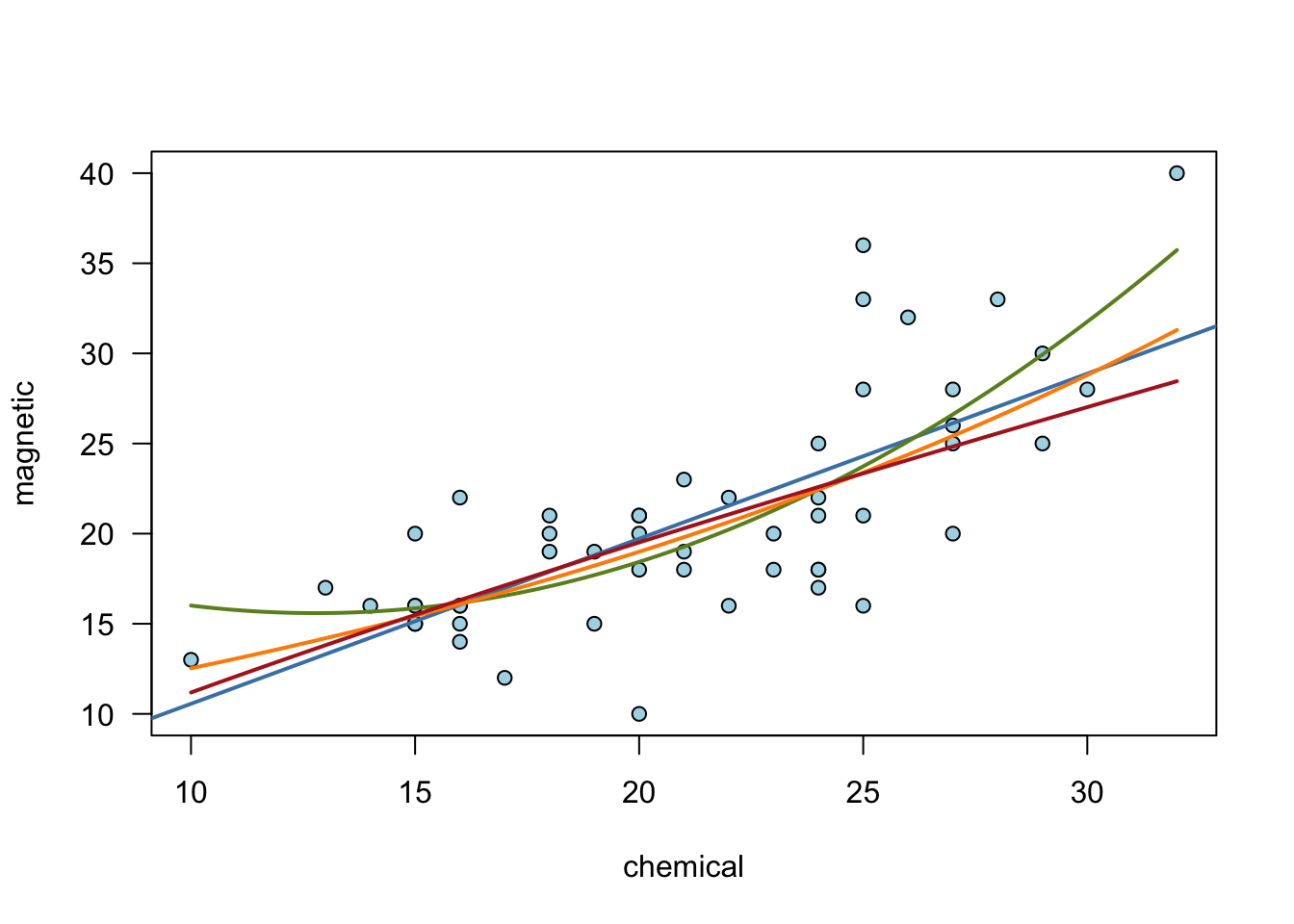
summary(linear)
Call:
lm(formula = magnetic ~ chemical)

Residuals:
    Min      1Q  Median      3Q     Max
-9.7180 -2.4653 -0.0549  2.0401 11.7032

Coefficients:
            Estimate Std. Error t value Pr(>|t|)
(Intercept)   1.4026     2.5843   0.543     0.59
chemical      0.9158     0.1190   7.695 4.38e-10 ***
---
Signif. codes:  0 '***' 0.001 '**' 0.01 '*' 0.05 '.' 0.1 ' ' 1

Residual standard error: 4.327 on 51 degrees of freedom
Multiple R-squared:  0.5372,    Adjusted R-squared:  0.5282
F-statistic: 59.21 on 1 and 51 DF,  p-value: 4.375e-10
Algorithm for leave-one-out cross-validation: 1. Set \(x_k\), \(y_k\) to be the test data. 2. Fit the model on \(n-1\) data points. 3. Compute the prediction error. 4. Estimate the mean of the squared prediction error.
n = nrow(ironslag)
elinear = equad = eexp = elog = numeric(n)
for (i in 1:n) {
    x = chemical[-i]
    y = magnetic[-i]
    xk = chemical[i]
    yk = magnetic[i]
    linear = lm(y ~ x)
    quad = lm(y ~ x + I(x^2))
    expfit = lm(log(y) ~ x)
    logfit = lm(log(y) ~ log(x))
    elinear[i] = (yk - predict(linear, data.frame(x = xk)))^2
    equad[i] = (yk - predict(quad, data.frame(x = xk)))^2
    eexp[i] = (yk - exp(predict(expfit, data.frame(x = xk))))^2
    elog[i] = (yk - exp(predict(logfit, data.frame(x = xk))))^2
}
round(cbind(
    mean(elinear),
    mean(equad),
    mean(eexp),
    mean(elog)
), 2)
[,1] [,2] [,3] [,4]
[1,] 19.56 17.85 18.44 20.45The output displays the mean squared prediction errors for linear, quadratic, exponential, and log-log models, providing a comparative performance measure for each model.
The following times represent hours between failures of air-conditioning equipment: 3, 5, 7, 18, 43, 85, 91, 98, 100, 130, 230, 487.
The log-likelihood function for \(\lambda\) is: \[ \log(L(\lambda)) = \sum_{i=1}^{n} \log(\lambda) - \lambda x_i \]
Taking the derivative with respect to \(\lambda\) and setting it to zero: \[ \frac{d}{d\lambda} \log(L(\lambda)) = \sum_{i=1}^{n} \frac{1}{\lambda} - x_i = 0 \]
Solving for \(\lambda\): \[ \hat{\lambda} = \frac{n}{\sum_{i=1}^{n} x_i} \]
times. Write R code to compute the MLE \(\hat{\lambda}\) based on times using the calculations in a) and perform \(B=200\) bootstraps to estimate the bootstrap bias and standard error of \(\hat{\lambda}\). Construct a histogram of the bootstrap replicates and overlay a vertical line at \(\hat{\lambda}\).times <- c(3, 5, 7, 18, 43, 85, 91, 98, 100, 130, 230, 487)
n <- length(times)
lambda_hat <- n / sum(times)
lambda_hat[1] 0.00925212B <- 200
lambda_b <- numeric(B)
for (b in 1:B) {
index <- sample(1:n, n, replace = TRUE)
lambda_b[b] <- n / sum(times[index])
}
bias <- mean(lambda_b) - lambda_hat
se <- sqrt(mean((lambda_b - mean(lambda_b))^2)) / sqrt(B)
hist(lambda_b, prob = TRUE, main = "Bootstrap Distribution of lambda", xlab = "lambda")
abline(v = lambda_hat, col = "red", lwd = 2)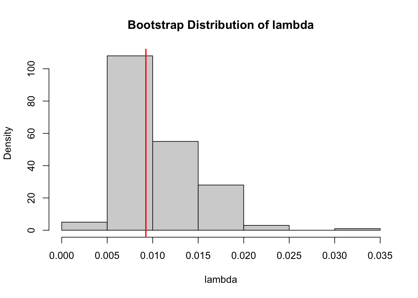
bias[1] 0.001045993se[1] 0.0002798803Suppose the sample \(X = (X_1, X_2, X_3)\) is collected from a distribution with mean \(\theta\) and we wish to perform the jackknife to estimate the bias of the sample mean \(\hat{\theta} = \bar{X} = \frac{X_1 + X_2 + X_3}{3}\).
For \(X = (X_1, X_2, X_3)\), the jackknife replicates are: - \(\hat{\theta}_{(1)} = \frac{X_2 + X_3}{2}\) - \(\hat{\theta}_{(2)} = \frac{X_1 + X_3}{2}\) - \(\hat{\theta}_{(3)} = \frac{X_1 + X_2}{2}\)
\[ \bar{\theta} = \frac{1}{3} \left( \frac{X_2 + X_3}{2} + \frac{X_1 + X_3}{2} + \frac{X_1 + X_2}{2} \right) \] \[ \bar{\theta} = \frac{1}{3} \left( \frac{2X_1 + 2X_2 + 2X_3}{6} \right) = \frac{X_1 + X_2 + X_3}{3} \]
\[ \text{bias}_{\text{jack}} = (n-1) (\bar{\theta} - \hat{\theta}) \] \[ \text{bias}_{\text{jack}} = 2 \left( \frac{X_1 + X_2 + X_3}{3} - \frac{X_1 + X_2 + X_3}{3} \right) = 0 \]
We consider a dataset containing the height (cm) of 20 randomly selected German men: 173, 183, 187, 179, 180, 186, 179, 196, 202, 198, 197, 185, 194, 185, 191, 182, 182, 187, 184, 186
\[ F_n(x) = \frac{1}{n} \sum_{i=1}^{n} I(X_i \leq x) \]
heights <- c(173, 183, 187, 179, 180, 186, 179, 196, 202, 198, 197, 185, 194, 185, 191, 182, 182, 187, 184, 186)
n <- length(heights)
B <- 200
# Standard normal bootstrap
real_mean <- mean(heights)
mean_b <- numeric(B)
for (b in 1:B) {
    index <- sample(1:n, n, replace = TRUE)
    mean_b[b] <- mean(heights[index])
}
bias <- mean(mean_b) - real_mean
se <- sqrt(mean((mean_b - mean(mean_b))^2)) / sqrt(B)
ci_sn <- c(real_mean - 1.96 * se, real_mean + 1.96 * se)

# Basic bootstrap
ci_bb <- c(2 * real_mean - quantile(mean_b, 0.975), 2 * real_mean - quantile(mean_b, 0.025))

# Percentile bootstrap
ci_pb <- c(quantile(mean_b, 0.025), quantile(mean_b, 0.975))

# Bootstrap t
values <- numeric(B)
for (b in 1:B) {
    index <- sample(1:n, n, replace = TRUE)
    mean_b[b] <- mean(heights[index])
    reps_for_se <- numeric(B)
    for (i in 1:B) {
        index <- sample(1:n, n, replace = TRUE)
        reps_for_se[i] <- mean(heights[index])
    }
    values[b] = (mean_b[b] - real_mean) / sd(reps_for_se)
}
t_quant <- quantile(values, c(0.975, 0.025))
ci_bt <- c(real_mean - t_quant[1] * se, real_mean - t_quant[2] * sd(reps_for_se))

cbind(ci_sn, ci_bb, ci_pb, ci_bt)
ci_sn ci_bb ci_pb ci_bt
97.5% 186.5842 183.5988 183.4975 186.5914
2.5% 187.0158 190.1025 190.0012 190.1948library(bootstrap)
data(law)
B <- 2000
n <- nrow(law)
thetahat <- cor(law$LSAT, law$GPA)
theta_b <- numeric(B)
for (b in 1:B) {
index <- sample(1:n, n, replace = TRUE)
theta_b[b] <- cor(law$LSAT[index], law$GPA[index])
}
# Calculate z0
z0 <- qnorm(sum(theta_b < thetahat) / B)
# Calculate a
jackknife_thetas <- numeric(n)
for (i in 1:n) {
jackknife_thetas[i] <- cor(law$LSAT[-i], law$GPA[-i])
}
theta_bar <- mean(jackknife_thetas)
a <- sum((theta_bar - jackknife_thetas)^3) / (6 * sum((theta_bar - jackknife_thetas)^2)^(3/2))
# Adjusted alpha values
alpha1 <- pnorm(z0 + (z0 + qnorm(0.025)) / (1 - a * (z0 + qnorm(0.025))))
alpha2 <- pnorm(z0 + (z0 + qnorm(0.975)) / (1 - a * (z0 + qnorm(0.975))))
# BCa confidence interval
ci_bca <- quantile(theta_b, c(alpha1, alpha2))
ci_bca0.4715224% 93.18272%
0.3620948 0.9392353 Implement the code in R to see if any errors occurred. Report and interpret the 95% CI BCa intervals.
Report the calculated values of \(z_0\) and \(a\), compare them to their values of 0 under no bias and no skewness, respectively. Visualize histograms of the bootstrap and jackknife replicates.
The usual bootstrap percentile interval uses \(\alpha_1 = 0.025\) and \(\alpha_2 = 0.975\) as the lower and upper cumulative probabilities for computation of the quantiles. Compare the BCa estimates of \(\alpha_1\) and \(\alpha_2\) to these. Use this comparison to explain how the BCa interval differs from the percentile interval.
a[1] -0.07567156z0[1] -0.1231352groups = c(rep(1:26, each = 2))
sample(groups) [1] 16 9 26 21 18 15 10 14 20 2 22 3 1 3 22 25 8 21 9 18 25 2 8 6 17
[26] 13 12 24 20 19 5 5 23 6 12 4 14 7 11 24 13 11 17 19 15 1 16 10 7 26
[51] 23 4