7 - Monte Carlo methods for Inference and Estimation
Author
Peter Nutter
Published
Sunday, May 19, 2024
These methods are sometimes called parametric bootstrapping.
Given a random sample \(X_1, X_2, \ldots, X_n\) from \(f\) collected to estimate \(\theta\), the estimator \(\hat{\theta}\) is a function of \(X_1, X_2, \ldots, X_n\). We can repeatedly draw samples from \(f\) to obtain a random sample of \(\hat{\theta}\) for \(J = 1, 2, \ldots, m\).
Example 7.1
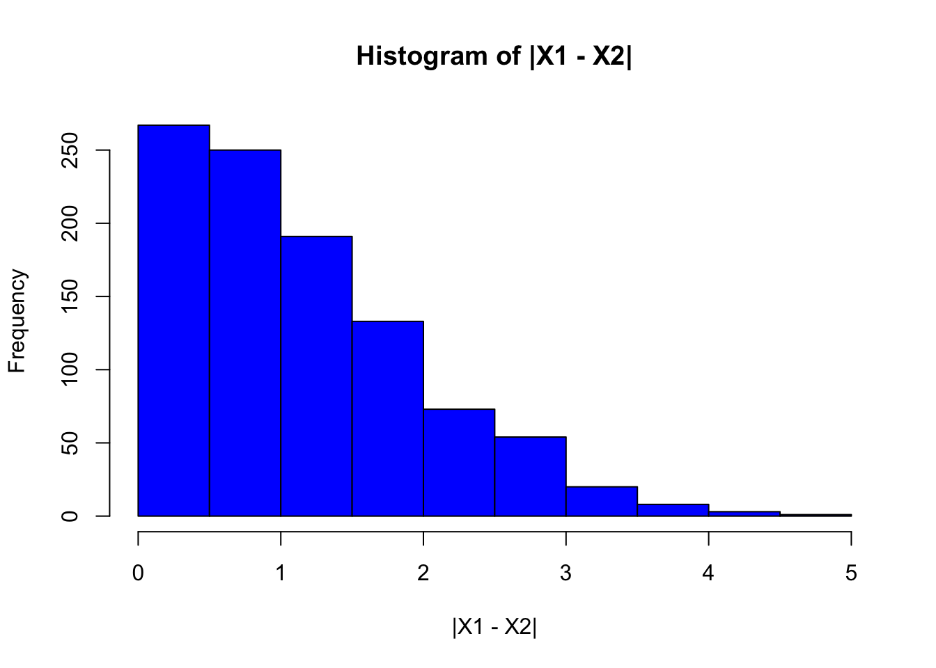
For \(X_1, X_2 \sim N(0, 1)\) iid, use Monte Carlo to estimate \(|X_1 - X_2|\). Given \(n = 2\), the estimator is \(\hat{\theta} = |X_1 - X_2|\).
set.seed(1981)m <-10^3normals <-matrix(rnorm(2* m), ncol =2)g <-abs(normals[, 1] - normals[, 2])mean_g <-mean(g)hist(g, col ="blue", main ="Histogram of |X1 - X2|", xlab ="|X1 - X2|")
# Variancese_g <-sd(g) /sqrt(m)cat(sprintf("Mean: %.4f\t Standard Error: %.4f\t", mean_g, se_g))
Mean: 1.1377 Standard Error: 0.0270
The histogram is useful for diagnosing the distribution of the estimator.
Estimating the Mean Squared Error of the Estimator
Given an estimator \(\hat{\theta}\), we draw a random sample of \(\hat{\theta}_j\) for \(j = 1, 2, \ldots, m\). \[
\text{MSE} = \frac{1}{m} \sum_{j=1}^{m} (\hat{\theta}_j - \theta)^2
\]
Example 7.2
Historically, trimmed means were used to estimate the mean of observed data when the potential for erroneous outliers was high. Today, the median is often used. The \(k\)-th level trimmed mean is the mean of the data after removing the \(k\) smallest and \(k\) largest values. \[
\bar{X}_{-k} = \frac{1}{n - 2k} \sum_{i=k+1}^{n-k} X_{(i)}
\] Write code to estimate the MSE of the first level trimmed mean of 20 observations from \(N(0, 1)\) to estimate the mean of the distribution.
set.seed(1982)n <-20m <-10^3normals <-matrix(rnorm(n * m), ncol = n)# Compute trimmed meantrimmed_mean <-apply(normals, 1, function(x) mean(sort(x)[2:(n-1)]))trimmed_mse <-mean((trimmed_mean -0)^2)trimmed_se_mse <-sd((trimmed_mean -0)^2) /sqrt(m)# Compute normal meannormal_mean <-apply(normals, 1, mean)normal_mse <-mean((normal_mean -0)^2)normal_se_mse <-sd((normal_mean -0)^2) /sqrt(m)# Compute medianmedian <-apply(normals, 1, median)median_mse <-mean((median -0)^2)median_se_mse <-sd((median -0)^2) /sqrt(m)# Display resultscat(sprintf("Trimmed Mean MSE: %.4f\tTrimmed Mean SE of MSE: %.4f\t", trimmed_mse, trimmed_se_mse))
Trimmed Mean MSE: 0.0511 Trimmed Mean SE of MSE: 0.0024
cat(sprintf("Normal Mean MSE: %.4f\tNormal Mean SE of MSE: %.4f\t", normal_mse, normal_se_mse))
Normal Mean MSE: 0.0498 Normal Mean SE of MSE: 0.0023
cat(sprintf("Median MSE: %.4f\tMedian SE of MSE: %.4f\t", median_mse, median_se_mse))
Median MSE: 0.0734 Median SE of MSE: 0.0035
The median throws out a lot of data, the trimmed mean is more robust to outliers, but the normal mean is the most efficient in this case.
The standard error of the MSE, \(\text{SE(MSE)}\), is also a Monte Carlo average \(\bar{g}(X)\) where \(\bar{g}(X) = (g(X) - \theta)^2\). \[
\text{SE(MSE)} = \sqrt{\frac{1}{m}} \sigma
\] where \(\sigma = \text{sd}((\hat{\theta}_j - \theta)^2)\).
Estimating Confidence Intervals
We can estimate \(100(1 - \alpha)\%\) confidence intervals for the mean \(\mu\) of \(X\): \[
\bar{X} \pm t_{n-1,1-\alpha/2} \frac{s}{\sqrt{n}}
\] where \(t_{n-1,1-\alpha/2}\) is the \(1 - \alpha/2\) quantile of the \(t\) distribution with \(n - 1\) degrees of freedom.
If the sample is large enough, greater than 30, we use the normal distribution instead of the \(t\) distribution: \[
\bar{X} \pm 1.96 \text{SE}(X)
\] This extends to \(\theta = \bar{g}(X)\) where \(\bar{g}(X)\) of iid data is computed by Monte Carlo sampling. The 95% confidence interval for \(\theta\) is \(\bar{g} \pm 2 \text{SE}(\bar{g})\).
If the sample is small, we must check the assumption of normality using QQ plots. We see that the confidence interval is also a random variable, a function of the random sample.
Theoretical Proof of Coverage for the Normal Distributed Single Sample Mean Case
Suppose that \(X_i \sim N(\mu, \sigma^2)\) iid for \(i = 1, \ldots, n\), or \(n\) is large so that by the central limit theorem, the sample mean \(\bar{X} \sim N(\mu, \sigma^2/n)\). Then \(T = \frac{\bar{X} - \mu}{s / \sqrt{n}} \sim t_{n-1}\), where \(s\) is the sample standard deviation.
Since the \(t\) distribution is symmetric about 0, with \(t_{n-1,1-\alpha/2}\) the upper \(1-\alpha/2\) quantile of the \(t_{n-1}\) distribution, by definition: \[
P(-t_{n-1,1-\alpha/2} \leq T \leq t_{n-1,1-\alpha/2}) = 1 - \alpha
\] Substituting \(T = \frac{\bar{X} - \mu}{s / \sqrt{n}}\) yields: \[
P\left(-t_{n-1,1-\alpha/2} \leq \frac{\bar{X} - \mu}{s / \sqrt{n}} \leq t_{n-1,1-\alpha/2}\right) = 1 - \alpha
\]\[
P\left(\bar{X} - t_{n-1,1-\alpha/2} \frac{s}{\sqrt{n}} \leq \mu \leq \bar{X} + t_{n-1,1-\alpha/2} \frac{s}{\sqrt{n}}\right) = 1 - \alpha
\]
Confidence intervals are invariant, so if \((\theta_L, \theta_U)\) is a confidence interval for \(\theta\), then generally \((g(\theta_L), g(\theta_U))\) is a confidence interval for \(g(\theta)\).
Note that a confidence interval \(C = (C_L, C_U)\) is a function of the data \(X_i, i = 1, \ldots, n\), and the theoretical proof relied upon the distributional assumptions of the data. In general, proving that a specified confidence interval obtains the correct confidence level is not easily done theoretically, but it is simple to do via Monte Carlo.
Monte Carlo Estimator of Confidence Level
Let \(X = X_1, \ldots, X_n\) iid from \(f\), which depends on fixed known parameters. \(\theta\) is the target parameter of the confidence interval \(C(X) = (C_L, C_U)\).
For \(j = 1, \ldots, m\), randomly draw \(X_j = (X_{1j}, \ldots, X_{nj})\) from \(f\) and compute \(C(X_j) = (C_{Lj}, C_{Uj})\). \[
\hat{\text{Conf}} = \frac{1}{m} \sum_{j=1}^{m} I(C(X_j) \text{ contains } \theta)
\] where \(I\) is the indicator function. \[
\text{SE}(\hat{\text{Conf}}) = \sqrt{\frac{\hat{\text{Conf}}(1 - \hat{\text{Conf}})}{m}}
\]
Verify by Simulation: Small Sample Normal Mean Case
We can see that if the data isn’t normally distributed and the sample size is small, we will not achieve the 95% confidence level. When we increase \(n\), the central limit theorem takes effect, and the means will be normally distributed.
Monte Carlo Methods for Inference
We assume a \(\theta \in \Theta\)
We specify a significance level \(\alpha\)
Hypothesis: \(H_0: \theta \in \Theta_0\) vs \(H_1: \theta \in \Theta_1\)
Where \(\Theta_0 \cap \Theta_1 = \emptyset\) and \(\Theta_0 \cup \Theta_1 = \Theta\)
Type 1 Error: Reject \(H_0\) when \(H_0\) is true
Type 2 Error: Fail to reject \(H_0\) when \(H_1\) is true
\(\alpha\) is the upper bound on the probability of a Type 1 error
\(p\)-value: The smallest \(\alpha\) for which \(H_0\) is rejected
Power: The probability of rejecting \(H_0\) when \(H_1\) is true
Often we have a two-sided point null hypothesis \(\theta = \theta_0\) vs \(\theta \neq \theta_0\)
The \(p\)-value is often explained as the probability of observing the data or more extreme data given \(H_0\) is true
Example 7.3
In a study of computer use, 1000 randomly selected Canadian internet users were asked how much time they spend using the internet in a typical week (Ipsos Reid, Aug. 9, 2005). The mean of the sample observations was 12.7 hours. The sample standard deviation was not reported but suppose it was 5 hours. Perform a hypothesis test with a significance level of 0.05 to decide if there is convincing evidence that the population mean for Canadian internet user weekly use is 12 hours.
We will use a two-sided t-test: \[
t = \frac{\bar{X} - \mu}{s / \sqrt{n}}
\]
mu <-12mean <-12.7s <-5n <-1000# Calculate the t-statistict <- (mean - mu) / (s /sqrt(n))# Calculate the p-valuep <-2*pt(-abs(t), df = n -1)cat(sprintf("t: %.4f\t p: %f\t", t, p))
t: 4.4272 p: 0.000011
We reject the null hypothesis that the mean is 12 hours.
Effect of Reduced Sample Size
n <-100t <- (mean - mu) / (s /sqrt(n))p <-2*pt(-abs(t), df = n -1)cat(sprintf("t: %.4f\t p: %f\t", t, p))
t: 1.4000 p: 0.164639
Monte Carlo Estimator for Type 1 Error
Let \(X_1, \ldots, X_n\) be from \(F_x\) which depends on fixed \(\theta\). We are testing \(H_0: \theta = \theta_0\) vs \(\theta \neq \theta_0\) based on a statistic \(T(X)\) and a determined rejection region defined by \(\alpha\). We estimate the type 1 error by Monte Carlo.
Algorithm
For \(j = 1\) to \(m\):
Draw \(X_j\)\(n\) random variables from \(F_x\) with \(\theta = \theta_0\)
Compute \(T_j = T(X_j)\)
Set \(I_j = 1\) if \(T_j\) is in the rejection region, 0 otherwise
Error = \(\frac{1}{m} \sum I_j\)
SE = \(\sqrt{\text{error} \cdot (1 - \text{error}) / m}\)
Example:
Using the previous example with \(n = 15\), consider two scenarios:
Data is normally distributed, so the distribution \(t_{14}\) under \(H_0\) is correct.
Data is not normally distributed, which along with the small sample size means the \(t\) distribution is not correct under \(H_0\).
Scenario 1: Normally Distributed Data with Variance 1
Power is the probability of rejecting \(H_0\) when \(H_1\) is true. In experiments, we often fix the level and find \(n\) ensuring the power is more than 80%. For simple scenarios, power can be solved analytically.
Algorithm
Draw \(X_j\) from \(F_x\) with \(\theta = \theta_1\)
Compute \(T_j = T(X_j)\)
Set \(I_j = 1\) if \(T_j\) is in the rejection region, 0 otherwise
Power = \(\frac{1}{m} \sum I_j\)
Example
Estimate the power of the previous test with \(\mu = 13\).
If the real \(\mu\) is 13, we have a 94% power of rejecting the null hypothesis.
Excersises
Monte Carlo Methods for Estimation
7.1-7.2 MC for Estimation
For \(X_1, \ldots, X_n\) iid \(N(\mu, \sigma^2)\), it can be shown that \((n-1)s^2/\sigma^2 \sim \chi^2_{n-1}\), where \(s^2\) is the sample variance and \(\chi^2_{n-1}\) is the chi-square distribution with \(n-1\) degrees of freedom. Use this to analytically derive the form of a two-sided \(100(1 - \alpha)\%\) confidence interval for \(\sigma^2\) based on the \(\alpha/2\) and \(1 - \alpha/2\) quantiles.
The confidence interval for \(\sigma^2\) is given by: \[
\left( \frac{(n-1)s^2}{\chi^2_{1-\alpha/2, n-1}}, \frac{(n-1)s^2}{\chi^2_{\alpha/2, n-1}} \right)
\]
Using (1), derive a \(100(1 - \alpha)\%\) confidence interval for \(\sigma\). By invariance, this is the square root of the CI for \(\sigma^2\).
The confidence interval for \(\sigma\) is given by: \[
\left( \sqrt{\frac{(n-1)s^2}{\chi^2_{1-\alpha/2, n-1}}}, \sqrt{\frac{(n-1)s^2}{\chi^2_{\alpha/2, n-1}}} \right)
\]
Write and implement R code to check the accuracy of the CI in (1) for \(\sigma^2\) by performing 100 simulations generating an iid sample of 10 \(N(0,1)\) observations to calculate a 95% CI. Compare the calculated confidence to 95% in terms of the standard error of the estimated confidence.
Example: Testing for Matthew McConaughey’s Support
The campaign office for Matthew McConaughey for Texas Governor plans to consult with and run a poll of 15 independent conservative Texas oil billionaires to see what proportion of them would pledge their support for Matthew. If less than 50% of the billionaires plan to support Matthew for Governor, then Matthew will cut his losses and abort his campaign. Therefore, the planned hypothesis test is \(H_0: \pi = 0.5\) vs \(H_A: \pi < 0.5\), where \(\pi\) is the proportion of Texas billionaires who would support Matthew.
The planned test statistic is \(Y\), the number of the 15 polled billionaires who vote to support Matthew. State the domain and distribution of \(Y\), including all parameters.
\(Y \sim \text{Binomial}(15, \pi)\) with domain \(0\) to \(15\).
The test procedure will be to reject \(H_0\) if \(Y \leq 3\). Write the R command to exactly calculate the significance level of this test, implement in R and report the result. Write the R code to perform simulation of the significance level and compare to the exact answer for 100, 1000, and 10,000 simulations.
For the test in (2), write the R command to calculate the power for \(\pi = 0.1\) and \(\pi = 0.4\), and implement in R. Compare these results and explain why one is higher than the other. Compute the standard error for the two power calculations based on 100 simulations.
The power is higher for \(\pi = 0.4\) compared to \(\pi = 0.1\) because it is easier to reject the null hypothesis when the true proportion is closer to 0.4 than when it is closer to 0.1, given the same threshold for rejection.