Monte Carlo Integration provides an unbiased estimator of the mean of functions \(g\) of random variables \(x\).

Given \(x \sim f(x)\) where \(f(x)\) is a continuous probability density function (PDF), we estimate \(\theta = \mathbb{E}[g(x)] = \int g(x) f(x) \, dx\) by random sampling.

For \(X_i \sim f(x)\) for \(i = 1, 2, 3, \ldots, n\):

\[ \hat{\theta} = \frac{1}{n} \sum_{i=1}^{n} g(X_i) \]

By the strong law of large numbers, \(\hat{\theta}\) converges to \(\theta\) as \(n \to \infty\) with probability 1. Statistical expectation is used to perform Monte Carlo integration.

Example

We aim to estimate \(\theta = \int_{0}^{1} g(x) \, dx\):

Since \(f(x) = U(0, 1)\) has the correct domain,
\(\theta = \mathbb{E}[g(x)]\) for \(x \sim U(0, 1) = \int_{0}^{1} g(x) \, dx\)

Algorithm:

Generate \(n\) random numbers \(X_i\) from \(U(0, 1)\).
Set \(\hat{\theta} = \frac{1}{n} \sum_{i=1}^{n} g(X_i)\).

Example 6.1

Write R code to compute a Monte Carlo estimate of \(\theta = \int_{0}^{1} e^{-x} \, dx\). Compare with the exact value.

n <- 10^6
x <- runif(n)
theta_hat <- mean(exp(-x))
theta_hat

[1] 0.6322769

exact <- 1 - exp(-1)
exact - theta_hat

[1] -0.0001563723

Change of Variable

To estimate \(\theta = \int_{a}^{b} g(x) \, dx\):

Change of variable: \(u = \frac{x - a}{b - a}, \quad du = \frac{1}{b - a} dx\)

Thus, \[ \theta = \int_{a}^{b} g(x) \, dx = \int_{0}^{1} (b - a) g(a + (b - a)u) \, du \]

\[ \hat{\theta} = \frac{1}{n} \sum_{i=1}^{n} g(a + (b - a) U_i) \]

Or generate \(U \sim U(a, b)\) and use \(f(x) = \frac{1}{b - a}\) for \(x \in [a, b]\).

Example

Write correct R code to compute a Monte Carlo estimate of \(\theta = \int_{2}^{4} e^{-x} \, dx\). Compare with the exact value.

n <- 10^6
x <- runif(n, 2, 4)
theta_hat <- (4 - 2) * mean(exp(-x))
theta_hat

[1] 0.1170434

Monte Carlo Integration for Unbounded Intervals

To estimate the CDF of the standard normal distribution:

\[ \Phi(x) = \int_{-\infty}^{x} \frac{1}{\sqrt{2\pi}} e^{-\frac{u^2}{2}} \, du \]

Using symmetry: \[ \Phi(x) = 1 - \Phi(-x) \]

Reduce the problem to: \[ \theta = \int_{0}^{x} \frac{1}{\sqrt{2\pi}} e^{-\frac{u^2}{2}} \, du \]

Use the Monte Carlo approach to estimate \(\Phi(x) = \int_{-\infty}^{x} \frac{1}{\sqrt{2\pi}} e^{-\frac{t^2}{2}} \, dt\) for a sequence of \(x\) ranging from 0.1 to 2.5 using a single random generation of 10,000 \(U(0, 1)\) random variables.

n <- 10^4
x <- seq(0.1, 2.5, 0.1)
estimate <- numeric(length(x))
u <- runif(n)
for (i in 1:length(x)) {
    g <- x[i] * exp(-(u * x[i])^2 / 2)
    estimate[i] <- 0.5 + mean(g) / sqrt(2 * pi)
}
true_cdf <- pnorm(x)
round(rbind(x, estimate, true_cdf), 3)

         [,1]  [,2]  [,3]  [,4]  [,5]  [,6]  [,7]  [,8]  [,9] [,10] [,11] [,12]
x        0.10 0.200 0.300 0.400 0.500 0.600 0.700 0.800 0.900 1.000 1.100 1.200
estimate 0.54 0.579 0.618 0.655 0.691 0.726 0.758 0.788 0.816 0.841 0.864 0.885
true_cdf 0.54 0.579 0.618 0.655 0.691 0.726 0.758 0.788 0.816 0.841 0.864 0.885
         [,13] [,14] [,15] [,16] [,17] [,18] [,19] [,20] [,21] [,22] [,23]
x        1.300 1.400 1.500 1.600 1.700 1.800 1.900 2.000 2.100 2.200 2.300
estimate 0.903 0.919 0.933 0.945 0.956 0.965 0.972 0.978 0.983 0.987 0.991
true_cdf 0.903 0.919 0.933 0.945 0.955 0.964 0.971 0.977 0.982 0.986 0.989
         [,24] [,25]
x        2.400 2.500
estimate 0.993 0.996
true_cdf 0.992 0.994

We want to generate the CDF of \(N(0, 1)\) using the normal random generator: \[ \Phi(x) = \mathbb{E}[1(X \leq x)] = \int_{-\infty}^{x} \frac{1}{\sqrt{2\pi}} e^{-\frac{u^2}{2}} \, du \]

Algorithm:

Generate \(n\) random numbers \(X_i\) from \(N(0, 1)\).
Set \(\hat{\theta} = \text{mean}(1(X_i \leq x))\) for \(i = 1, 2, 3, \ldots, n\).

This method can generate a CDF for any distribution that we can generate random numbers from, though it is less efficient than sampling from the uniform distribution.

Standard Error of Monte Carlo Sample Mean (Continuous Case)

Given \(X \sim f(x)\) and \(g(x)\) not being a probability but having a range on the real line, we are interested in \(\theta = \mathbb{E}[g(x)]\).

By generating from \(f(x)\) and calculating the sample mean of \(g(x)\), the variance of \(g(X)\) is:

\[ \text{var}(\hat{g}) = \frac{\text{var}(g(X))}{n} \]

The standard error is:

\[ \text{SE} = \sqrt{\frac{\text{var}(g(X))}{n}} \]

We estimate the standard error by the sample standard deviation of the \(g(x)\) values.

Standard Error: Proportion Case

For \(\theta = \mathbb{E}[g(x)] = p\):

\[ \text{SE} = \sqrt{\frac{p(1 - p)}{n}} \]

with the upper bound \(\frac{0.5}{n}\). This estimate is used if the estimate is a proportion instead of using the one with variance.

Confidence Intervals

By the central limit theorem:

\[ \frac{\hat{\theta} - \mathbb{E}[\hat{\theta}]}{\text{SE}} \to N(0, 1) \text{ in distribution as } n \to \infty \]

To develop a 95% confidence interval for \(\theta\):

\[ P(-1.96 < \frac{\hat{\theta} - \theta}{\text{SE}} < 1.96) = 0.95 \] \[ P(\hat{\theta} - 1.96 \text{SE} < \theta < \hat{\theta} + 1.96 \text{SE}) = 0.95 \]

Thus, \(\hat{\theta} \pm 1.96 \text{SE}\) is a 95% confidence interval for \(\theta\).

For a general interval of \(100(1 - \alpha)\%\):

\[ \hat{\theta} \pm z_{\alpha/2} \text{SE} \]

where \(z_{\alpha/2}\) is the \(1 - \alpha/2\) quantile of the standard normal distribution.

Variance Reduction

Efficiency

If \(\theta_1\) and \(\theta_2\) are two unbiased estimators of \(\theta\):

\(\theta_1\) is more efficient than \(\theta_2\) if \(\text{var}(\theta_1) < \text{var}(\theta_2)\)

The percent reduction in variance by using \(\theta_1\) is:

\[100 \times \frac{\text{var}(\theta_2) - \text{var}(\theta_1)}{\text{var}(\theta_2)} \]

Sample Size Calculation

Starting with an estimate of \(\sigma < \epsilon\):

\[ n > \frac{\sigma^2}{\epsilon^2} \]

Our goal is to reduce variance while preserving unbiasedness.

Importance Sampling

Algorithm

To estimate \(\theta = \mathbb{E}[g(x)] = \int_{a}^{b} g(x) \, dx\), we use the following steps:

Generate \(X_1, X_2, \ldots, X_n\) from \(U(a, b)\).
Calculate \(\hat{\theta} = \frac{1}{n} \sum_{i=1}^{n} g(X_i)\).

This method can be inefficient if \(g(x)\) is small in some regions of the domain of \(f(x)\) and large in others. Importance sampling improves efficiency by replacing the uniform density with a density that more closely resembles the shape of \(g(x)\).

Importance Functions

We aim to find a density \(f_x\) where \(f_x > 0\) and \(g(x) \neq 0\), which is easy to generate from. This density is called the importance function. If \(X \sim f_x\), let \(Y = \frac{g(x)}{f(x)}\); then \(Y\) is an unbiased estimator of \(\theta\).

\[ \mathbb{E}_Y(Y) = \mathbb{E}_X \left( \frac{g(x)}{f(x)} \right) = \int_{a}^{b} g(x) f(x) \,/ f(x) \, dx = \theta \]

Generate \(X_1, X_2, \ldots, X_n\) from \(f_x\):

\[ \hat{\theta} = \frac{1}{n} \sum_{i=1}^{n} \frac{g(X_i)}{f(X_i)} \]

Choosing the Right Density

The variance of \(\hat{\theta}\) is:

\[ \text{var}(\hat{\theta}) = \frac{\text{var}\left(\frac{g(X)}{f(X)}\right)}{n} \]

We want to choose \(f\) such that the variance of \(g/f\) is finite and small. The best approach is to mimic the shape of \(g(x)\) as closely as possible, making \(g/f\) approximately constant, which has zero variance.

Example

Suppose we want to estimate:

\[ \theta = \int_{0}^{1} \frac{e^{-x}}{1 + x^2} \, dx \]

Comparing Functions

Consider the following functions:

\(f_1(x) = 1\) for \(0 < x < 1\)
\(f_2(x) = e^{-x}\) for \(0 < x < \infty\)
\(f_3(x) = (1 + x^2)^{-1}/\pi\) for \(-\infty < x < \infty\)
\(f_4(x) = e^{-x}/(1 - e^{-1})\) for \(0 < x < 1\)
\(f_5(x) = 4(1 + x^2)^{-1}/\pi\) for \(0 < x < 1\)

x <- seq(0, 1, .01)
f1 <- rep(1, length(x))
f2 <- exp(-x)
f3 <- 1 / ((1 + x^2) * pi)
f4 <- exp(-x) / (1 - exp(-1))
f5 <- 4 / ((1 + x^2) * pi)
g <- exp(-x) / (1 + x^2)
w <- 2

# We want to approximate the function g(x) = exp(-x)/(1+x^2)
plot(x, g, type="l", main="", ylab="", ylim=c(0, 2), las=1, lwd=w)
lines(x, f1, col="turquoise", lwd=w)
lines(x, f2, col="salmon", lwd=w)
lines(x, f3, col="royalblue", lwd=w)
lines(x, f4, col="lightpink2", lwd=w)
lines(x, f5, col="limegreen", lwd=w)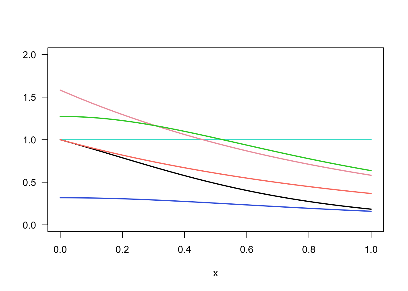

Visualizing the Ratios of the Functions

plot(x, g, type="l", main="", ylab="", ylim=c(0, 3.2), col="turquoise", las=1, lwd=w)
lines(x, g / f2, col="salmon", lwd=w)
lines(x, g / f3, col="royalblue", lwd=w)
lines(x, g / f4, col="lightpink2", lwd=w)
lines(x, g / f5, col="limegreen", lwd=w)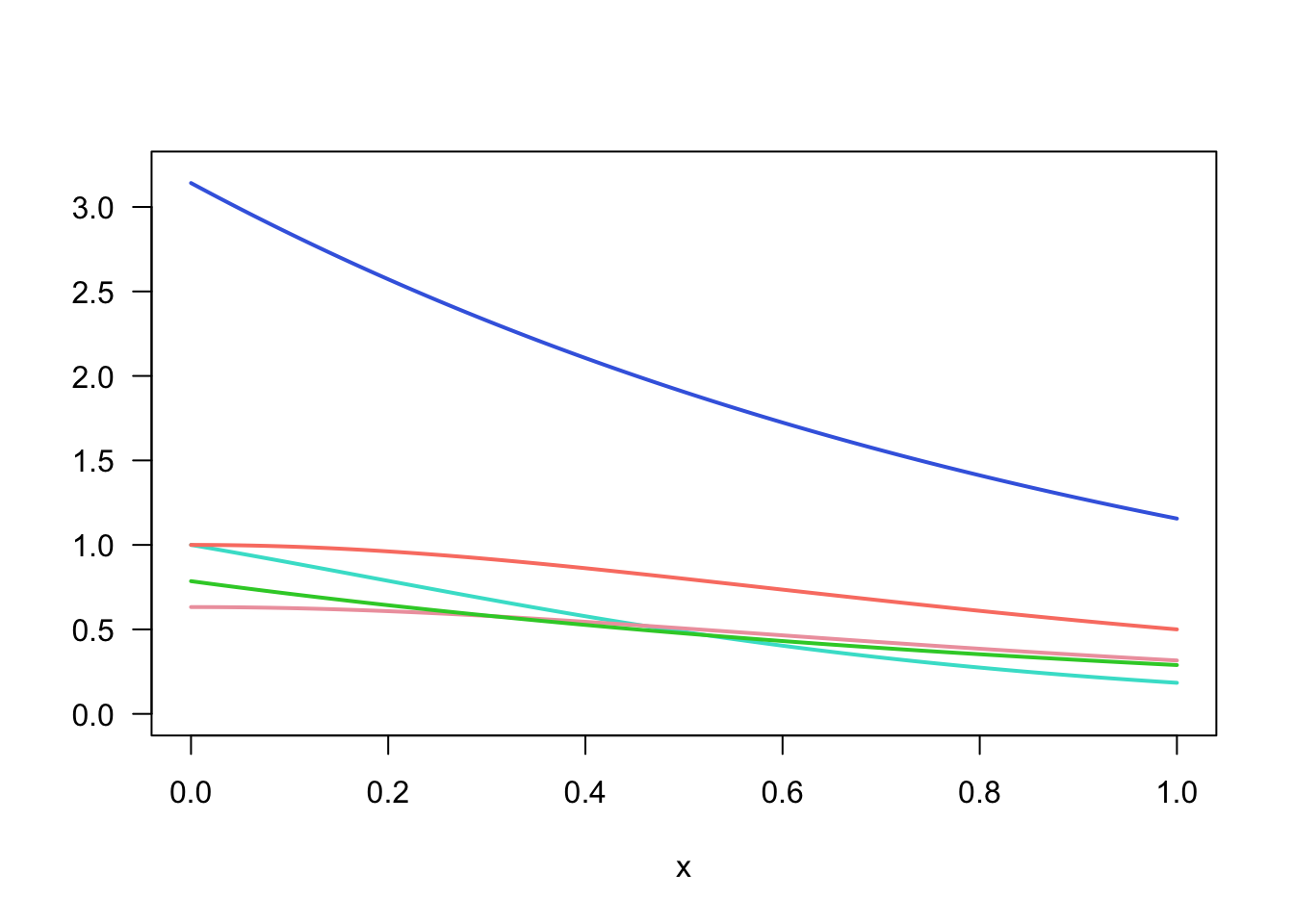

\(f_3\) is the worst. For each function, generate samples and compare the standard errors.

n <- 10^4

g <- function(x) exp(-x) / (1 + x^2) * (x > 0) * (x < 1)
thetas <- ses <- numeric(5)

# Uniform distribution
x <- runif(n)
gf_ratio <- g(x)
ses[1] <- sd(gf_ratio) / sqrt(n)
thetas[1] <- mean(gf_ratio)
hist(gf_ratio)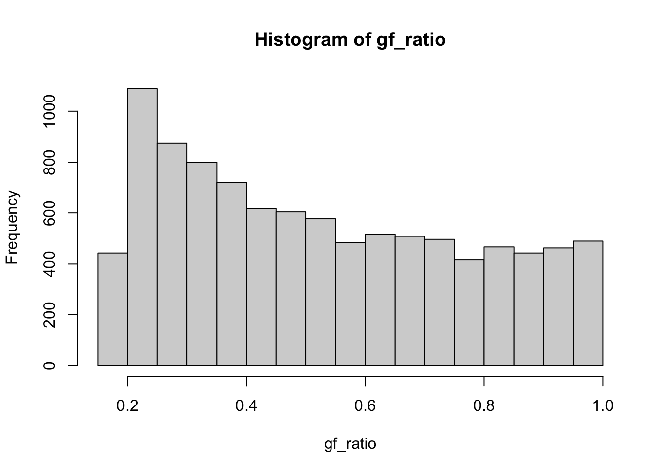

Exponential Distribution

f2 <- rexp(n, 1)
gf_ratio <- g(f2) / exp(-f2)
ses[2] <- sd(gf_ratio) / sqrt(n)
thetas[2] <- mean(gf_ratio)
hist(gf_ratio)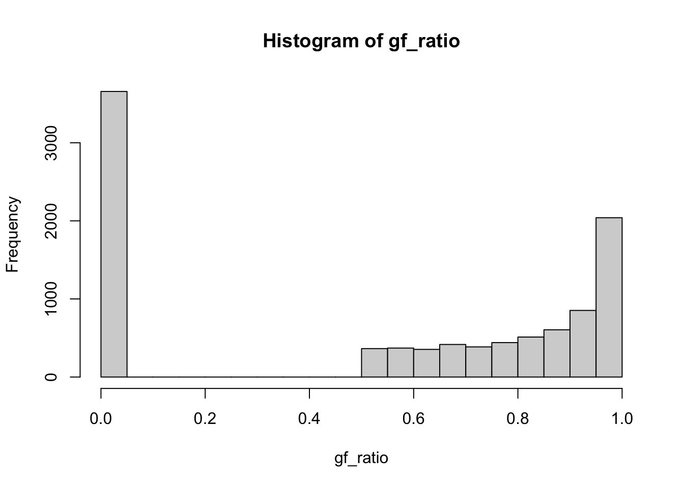

cbind(thetas, ses)

        thetas         ses
[1,] 0.5249117 0.002434840
[2,] 0.5280543 0.004189791
[3,] 0.0000000 0.000000000
[4,] 0.0000000 0.000000000
[5,] 0.0000000 0.000000000

\(t\) Distribution with 1 Degree of Freedom

f3 <- rt(n, 1)
f3[f3 < 0] <- 0
f3[f3 > 1] <- 1
gf_ratio <- g(f3) / dt(f3, 1)
ses[3] <- sd(gf_ratio) / sqrt(n)
thetas[3] <- mean(gf_ratio)
hist(gf_ratio)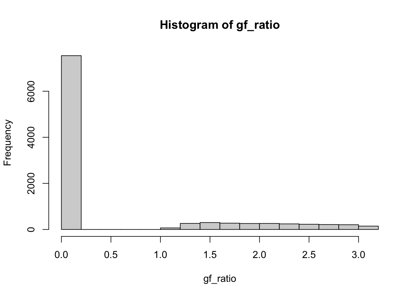

cbind(thetas, ses)

        thetas         ses
[1,] 0.5249117 0.002434840
[2,] 0.5280543 0.004189791
[3,] 0.5118427 0.009397544
[4,] 0.0000000 0.000000000
[5,] 0.0000000 0.000000000

summary(gf_ratio)

   Min. 1st Qu.  Median    Mean 3rd Qu.    Max. 
 0.0000  0.0000  0.0000  0.5118  0.0000  3.1390

# Percentage of zero values
sum(gf_ratio == 0) / n

[1] 0.7543

Generating from \(f_4\) Using the Inverse Transform Method

Algorithm:

Generate \(U \sim U(0, 1)\)
Set \(X = F_X^{-1}(U)\)
\(f_4(x) = \frac{e^{-x}}{1 - e^{-1}}\)
\(F_X = \frac{1 - e^{-x}}{1 - e^{-1}}\)
\(x = -\log(1 - u(1 - e^{-1}))\)

u <- runif(n)
f4 <- -log(1 - u * (1 - exp(-1)))
gf_ratio <- g(f4) / (exp(-f4) / (1 - exp(-1)))
ses[4] <- sd(gf_ratio) / sqrt(n)
thetas[4] <- mean(gf_ratio)
hist(gf_ratio)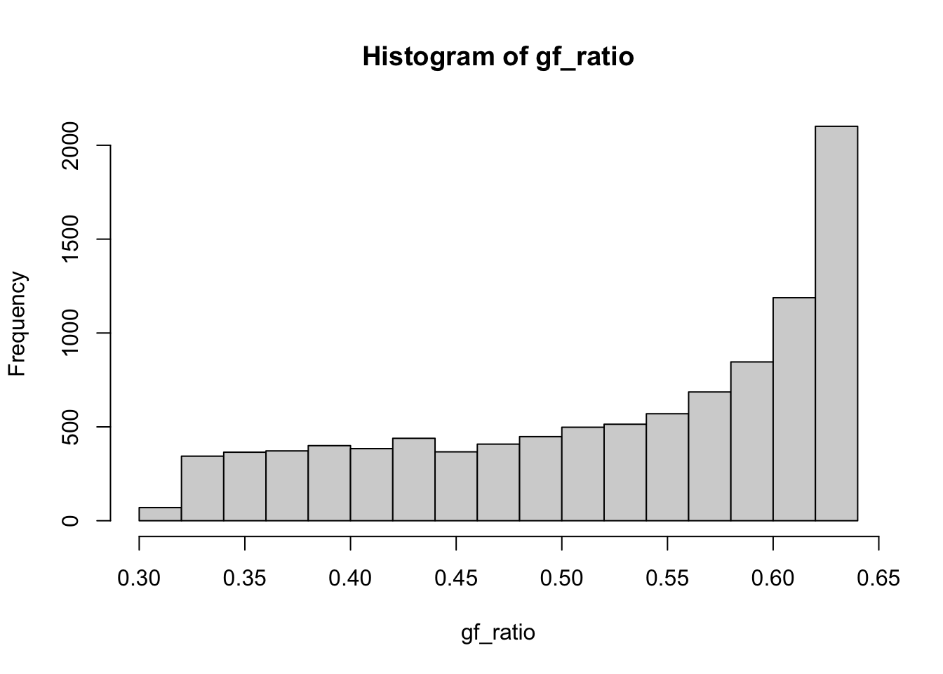

cbind(thetas, ses)

        thetas          ses
[1,] 0.5249117 0.0024348399
[2,] 0.5280543 0.0041897912
[3,] 0.5118427 0.0093975442
[4,] 0.5256000 0.0009666557
[5,] 0.0000000 0.0000000000

Truncating exponential density to (0, 1) and plotting the histogram improves efficiency.

hist(f4)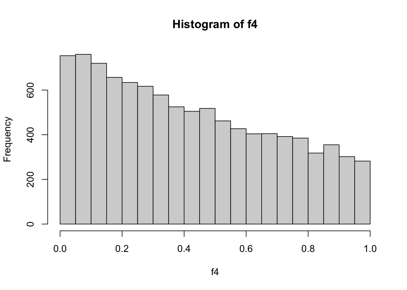

\(f_5\) is the Cauchy Distribution Truncated to (0, 1)

Using the inverse transform method:

\[ f_5 = 4(1 + x^2)^{-1} / \pi \]

\[ F_X = \frac{4 \arctan(x)}{\pi} \]

\[ x = \tan\left(\frac{\pi}{4} u\right) \]

u <- runif(n)
f5 <- tan(pi / 4 * u)
gf_ratio <- g(f5) / (4 / ((1 + f5^2) * pi))
ses[5] <- sd(gf_ratio) / sqrt(n)
thetas[5] <- mean(gf_ratio)
hist(gf_ratio)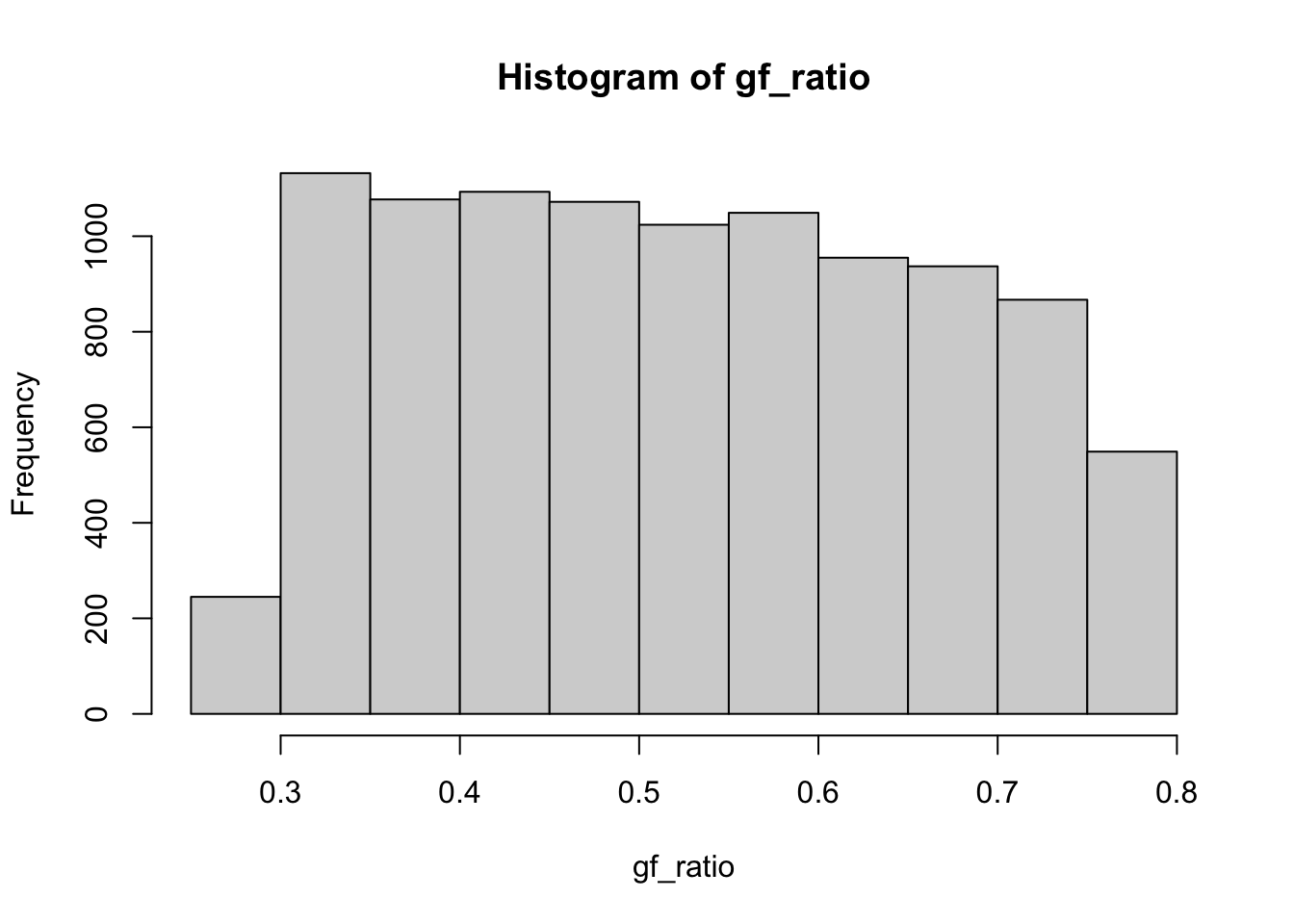

cbind(thetas, ses)

        thetas          ses
[1,] 0.5249117 0.0024348399
[2,] 0.5280543 0.0041897912
[3,] 0.5118427 0.0093975442
[4,] 0.5256000 0.0009666557
[5,] 0.5238577 0.0014099314

Main Takeaways

When possible, choose a function with the same domain as the integral to improve the efficiency of importance sampling.

Excercise 6

Importance Sampling Example

1. Consider the integral \(\theta = \int_{0}^{0.5} e^{-x} \, dx\)

a) Write the formula for the integral and evaluate it. Provide an algorithm to generate a MC estimate \(\hat{\theta}\) of \(\theta\) by sampling \(m\) iid \(Unif(0,0.5)\) random variables, showing all work.

The integral can be written as: \[ \theta = \int_{0}^{0.5} e^{-x} \, dx \]

Evaluating the integral: \[ \theta = \left[-e^{-x}\right]_{0}^{0.5} = 1 - e^{-0.5} \]

Algorithm:

Generate \(m\) random variables \(U_1, U_2, \ldots, U_m \sim Unif(0,0.5)\).
Calculate \(\hat{\theta} = \frac{1}{m} \sum_{i=1}^{m} \frac{e^{-U_i}}{0.5}\).

R code to estimate \(\hat{\theta}\):

n <- 100
u <- runif(n, 0, 0.5)
g <- function(x) exp(-x) * (x > 0) * (x < 0.5)
theta_hat <- 1/2 * mean(g(u))
theta_hat
theta <- 1 - exp(-0.5)
theta

b) Derive the theoretical variance of \(\hat{\theta}\) in (a) analytically and provide the numerical result for \(m = 100\).

The theoretical variance of \(\hat{\theta}\) is given by:

\[ \text{Var}(\hat{\theta}) = \frac{\text{Var}\left(\frac{e^{-X}}{0.5}\right)}{m} \] For \(X \sim Unif(0, 0.5)\): \[ \text{Var}\left(\frac{e^{-X}}{0.5}\right) = \frac{1}{0.5^2} \left(\mathbb{E}[e^{-2X}] - (\mathbb{E}[e^{-X}])^2\right) \] With \(\mathbb{E}[e^{-X}] = \frac{1 - e^{-0.5}}{0.5}\) and \(\mathbb{E}[e^{-2X}] = \frac{1 - e^{-1}}{1}\): \[ \text{Var}\left(\frac{e^{-X}}{0.5}\right) = 4 \left(\frac{1 - e^{-1}}{1} - \left(\frac{1 - e^{-0.5}}{0.5}\right)^2\right) \] For \(m = 100\): \[ \text{Var}(\hat{\theta}) = \frac{4 \left(\frac{1 - e^{-1}}{1} - \left(\frac{1 - e^{-0.5}}{0.5}\right)^2\right)}{100} \]

c) Write down another MC estimator \(\theta^*\) by sampling from the exponential distribution with density \(f(x) = \lambda e^{-\lambda x}\) for \(\lambda > 0\), \(x > 0\).

For \(\lambda = 2\), \(f(x) = 2e^{-2x}\) for \(x > 0\). The estimator is:

\[ \theta^* = \frac{1}{m} \sum_{i=1}^{m} \frac{e^{-X_i}}{2e^{-2X_i}} \] where \(X_i \sim \text{Exp}(2)\).

d) Derive the theoretical variance of \(\theta^*\) in (c) analytically and provide the numerical result for \(m = 100\).

The theoretical variance of \(\theta^*\) is given by:

\[ \text{Var}(\theta^*) = \frac{\text{Var}\left(\frac{e^{-X}}{2e^{-2X}}\right)}{m} \] For \(X \sim \text{Exp}(2)\): \[ \text{Var}\left(\frac{e^{-X}}{2e^{-2X}}\right) = \text{Var}\left(\frac{1}{2} e^{X}\right) \] With \(\mathbb{E}[e^{X}] = \frac{1}{1 - (-1)} = 2\) and \(\mathbb{E}[e^{2X}] = \frac{1}{1 - (-2)} = \frac{2}{3}\): \[ \text{Var}\left(\frac{1}{2} e^{X}\right) = \frac{1}{4} \left(\mathbb{E}[e^{2X}] - (\mathbb{E}[e^{X}])^2\right) = \frac{1}{4} \left(\frac{2}{3} - 4\right) = \frac{1}{4} \left(\frac{2}{3} - 4\right) \] For \(m = 100\): \[ \text{Var}(\theta^*) = \frac{\frac{1}{4} \left(\frac{2}{3} - 4\right)}{100} \]

e) Write the expression for the ratio of theoretical variances from (b) and (d): \(\frac{\text{Var}(\hat{\theta})}{\text{Var}(\theta^*)}\), and evaluate the result numerically. Interpret the result. Which estimator is more efficient? Explain intuitively why.

The ratio of the theoretical variances is:

\[ \frac{\text{Var}(\hat{\theta})}{\text{Var}(\theta^*)} \]

Evaluating the ratio numerically will show which estimator is more efficient. Generally, an estimator that samples more closely from the target distribution \(g(x)\) will be more efficient, as it reduces the variance.

f) Write and implement R code to estimate \(\hat{\theta}\) and \(\theta^*\) and their sample variances using \(m = 100\). Compare to the analytically derived results.

R code to estimate \(\hat{\theta}\):

n <- 100
u <- runif(n, 0, 0.5)
g <- function(x) exp(-x) * (x > 0) * (x < 0.5)
theta_hat <- 1/2 * mean(g(u))
theta_hat
theta <- 1 - exp(-0.5)
theta

# Sample variance
var_theta_hat <- var(1/2 * g(u)) / n
var_theta_hat

R code to estimate \(\theta^*\):

set.seed(25)
n <- 100
lambda <- 2
x <- rexp(n, rate = lambda)
g_exp <- function(x) exp(-x) * (x > 0) * (x < 0.5)
theta_star <- mean(g_exp(x) / (lambda * exp(-lambda * x)))
theta_star

# Sample variance
var_theta_star <- var(g_exp(x) / (lambda * exp(-lambda * x))) / n
var_theta_star

Importance Sampling

1a) Let \(\hat{\theta}_{f_{IS}}\) be an importance sampling estimator of \(\theta = \int g(x) \, dx\) with \(f(x)\) being the importance function probability density. Prove that if \(\frac{g(x)}{f(x)}\) is bounded, then the variance of \(\hat{\theta}_{f_{IS}}\) is finite.

If \(\frac{g(x)}{f(x)}\) is bounded, say by \(M\), then:

\[ \left(\frac{g(x)}{f(x)}\right)^2 \leq M^2 \] Hence, the second moment is bounded: \[ \mathbb{E}\left[\left(\frac{g(X)}{f(X)}\right)^2\right] < \infty \] Thus, the variance is finite.

b) Consider the integral \(\int_{1}^{\infty} \frac{x^2}{\sqrt{2\pi}} e^{-x^2/2} \, dx\). Write down the algorithm to calculate an estimate \(\hat{\theta}\) of this integral by using the importance sampling method with the re-scaled \(Exp(1)\) density \(f(x) = e^{-x+1}\), \(x > 1\), as the importance function.

Algorithm:

Generate \(X_1, X_2, \ldots, X_n\) from the re-scaled \(Exp(1)\) density: \(X = 1 - \log(U)\), \(U \sim Unif(0,1)\).
Calculate the importance sampling estimate: \[ \hat{\theta} = \frac{1}{n} \sum_{i=1}^{n} \frac{g(X_i)}{f(X_i)} \] where \(g(x) = \frac{x^2}{\sqrt{2\pi}} e^{-x^2/2}\) and \(f(x) = e^{-x+1}\).

c) Write R code to implement the algorithm in (b) and use it to calculate \(\hat{\theta}\) using 1000 samples. Report the standard deviation of \(\frac{g(x)}{f(x)}\).

set.seed(25)
n <- 1000
u <- runif(n)
x <- 1 - log(u)
g <- function(x) (x^2 / sqrt(2 * pi)) * exp(-x^2 / 2)
f <- function(x) exp(-x + 1)
gf_ratio <- g(x) / f(x)
theta_hat <- mean(gf_ratio)
theta_hat
sd_theta_hat <- sd(gf_ratio)
sd_theta_hat