3 - Generating Random Variables

Introduction

• Assume we have a generator for uniform \(U(0,1)\).
• In R, it’s runif(n):

round(runif(5, 1, 2), 2)

[1] 1.09 1.67 1.47 1.66 1.90

• The CDF of \(U(0,1)\) is \(F(x) = x\).
• Quantile \(x_q = q\) for \(U(0,1)\).
• Discrete sampling:

sample(1:100, size = 6, replace = FALSE)

[1] 10 23 59 29 61 58

x <- sample(1:3, size = 10, replace = TRUE, prob = c(.2, .3, .5))
table(x)

x
1 2 3 
3 3 4 

Some R Distributions

• p: cumulative distribution
• r: random variable
• d: probability distribution
• q: quantile

Distribution	R Tag	Parameters
Beta	beta	shape1, shape2
Binomial	binom	size, prob
Chi-squared	chisq	df
Exponential	exp	rate
F	f	df1, df2
Gamma	gamma	shape, rate or scale
Geometric	geom	prob
Lognormal	lnorm	meanlog, sdlog
Negative Binomial	nbinom	size, prob
Normal	norm	mean, sd
Poisson	pois	lambda
Student’s t	t	df
Uniform	unif	min, max

Generate \(U(a, b)\) from \(U(0, 1)\)

• Transformation: \[ y = a + (b-a)x \]

Check:

a <- 2
b <- 4
hist(runif(1000, a, b))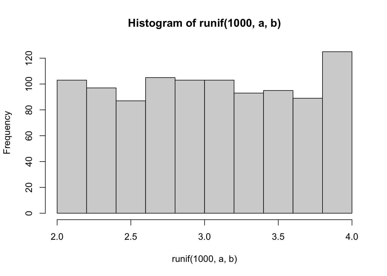

hist(a + (b - a) * runif(1000), prob = TRUE, col = "turquoise1", las = 1)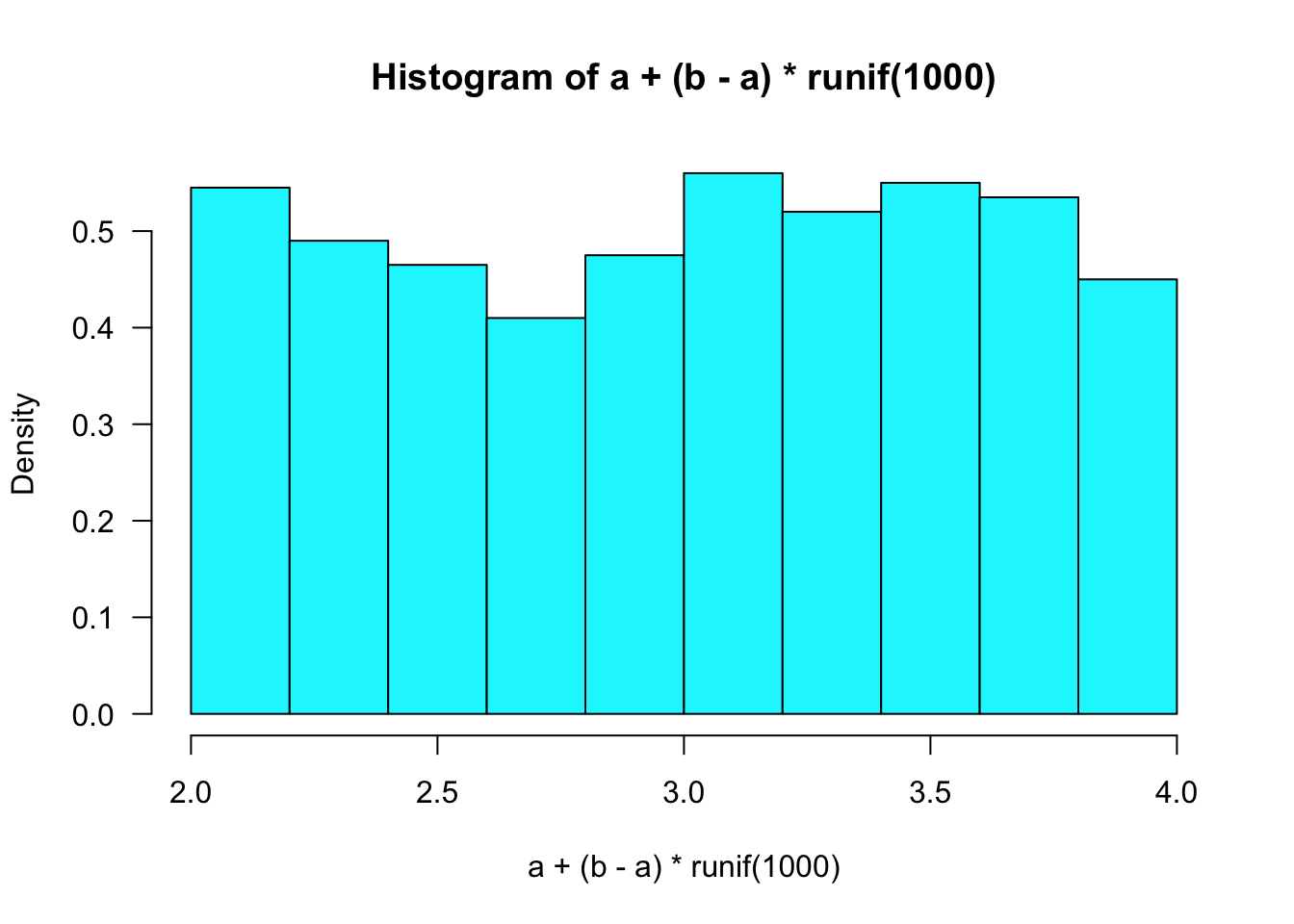

• We can check that the density is the same by PDF or by CDF equality.

Density Transformation

• For \(x\) in \(\mathbb{R}^n\): \[ y = g(x) \text{ needs to be 1-to-1} \] \[ \frac{dx}{dy} = \text{Jacobian} = \frac{g^{-1}(y)}{dy} \] \[ f_Y(y) = f_X(g^{-1}(y)) \left| \frac{dx}{dy} \right| \]

Inverse Transform Method

• Let \(X\) be a continuous random variable with CDF \(F_X\) (assume for simplicity \(F_X\) is strictly increasing).

  \[ F_X(X) \sim U(0,1) \]

Proof: - CDF of \(U(0,1)\) is \(F_U(u) = u\) \[ P(F_X(X) \leq u) = P(X \leq F_X^{-1}(u)) = F_X(F_X^{-1}(u)) = u \]

Method: - Generate random uniform \(U \sim U(0,1)\). - Set \(X = F_X^{-1}(U)\).

• Algorithm only works if we can obtain \(F^{-1}\).
• Generated \(X\) has a CDF \(F_X\): \[ P(X \leq x) = P(F_X^{-1}(U) \leq x) = P(U \leq F_X(x)) = F_X(x) \]
• This also works for a non-strictly increasing CDF if we define the quantile with an infimum.

Example: Generate from density \(3x^2\) for \(x\) in \([0, 1]\). - \(F_X = x^3\) - \(x = F_X^{-1}(u)\) - \(x = u^{1/3}\)

Code:

n <- 1000
u <- runif(n)
x <- u^(1 / 3)
hist(x, prob = TRUE, las = 1)
y <- seq(0, 1, 0.1)
lines(y, 3 * y^2, lwd = 2, add = T)

Warning in plot.xy(xy.coords(x, y), type = type, ...): "add" is not a graphical
parameter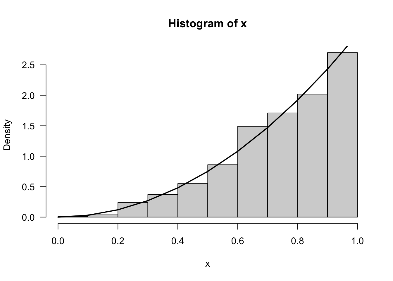

Exponential Example

• \(f_X = \lambda e^{-\lambda x}\) for \(x\) in \([0, \infty)\).
• \(F_X(x) = 1 - e^{-\lambda x}\)
• \(F(x) = u\)
• \(x = -\log(1 - u) / \lambda\)

Algorithm:

n <- 1000
lambda <- 1
u <- runif(n)
x <- -log(1 - u) / lambda

hist(x, prob = TRUE)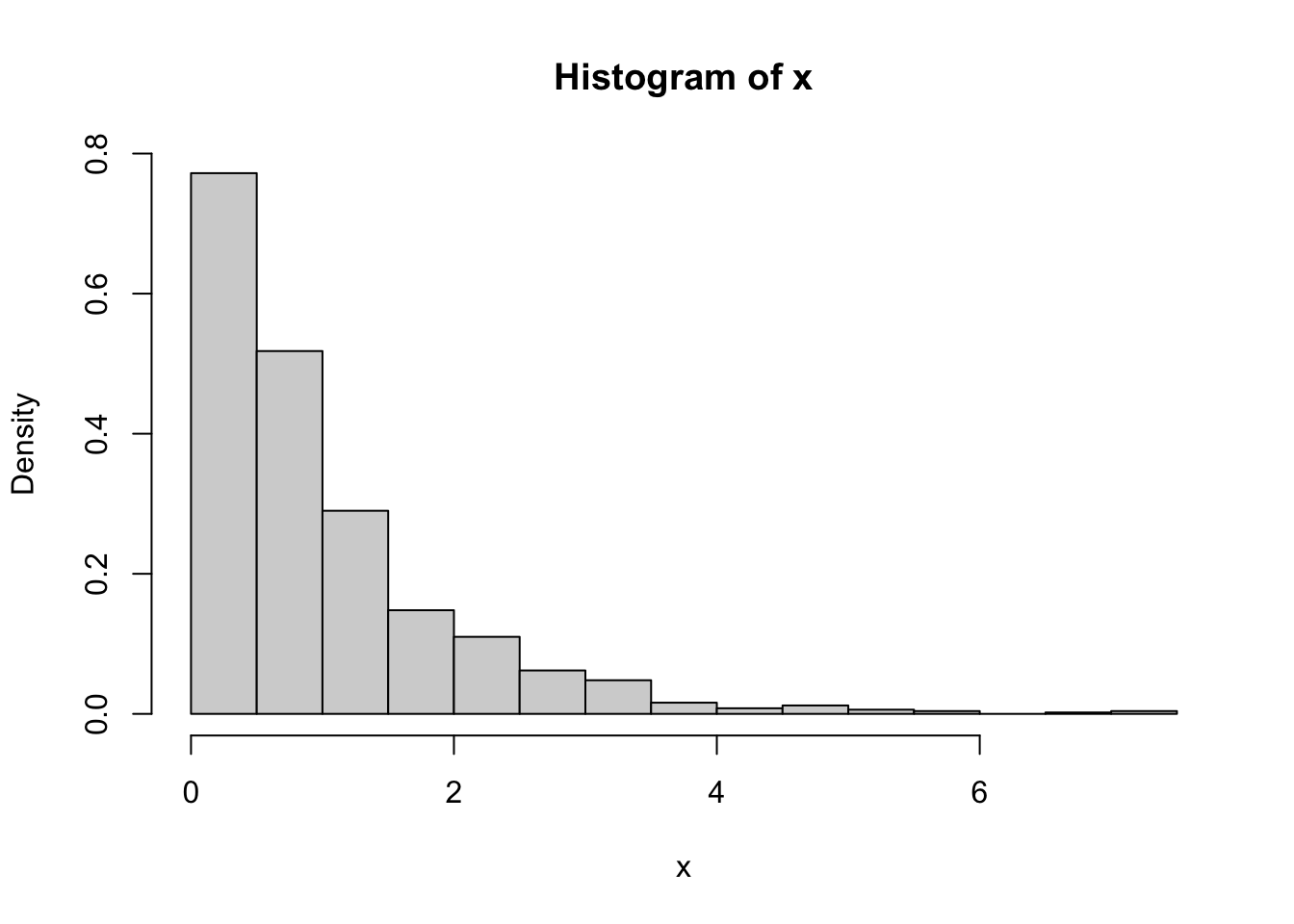

Note: In practice, \(1 - u\) is often used to avoid issues with \(u = 0\).

Inverse Transform Method for Discrete Random Variables

• Let \(X\) be a discrete random variable with \(x_{i-1} < x_i < x_{i+1}\), which are the points of discontinuity. \[ F_X^{-1}(u) = x_i \quad \text{where} \quad F_X(x_{i-1}) < u \leq F_X(x_i) \]

Algorithm: - Generate random uniform \(U \sim U(0,1)\). - Set \(X = x_i\) if \(F_X(x_{i-1}) < U \leq F_X(x_i)\).

Example: \(X\) Bernoulli(p) - \(P(X=0) = 1-p\) - \(P(X=1) = p\) - \(F(0) = 1-p\) - \(F(1) = 1\) \[ X = I(1-p < U \leq 1) = I(1-p < U) \]

We discretize the quantile line in the proportion of the discrete probabilities.

Acceptance-Rejection Method

• We want to generate from a density \(f(y)\) that has a complicated form and other methods don’t work.
  • We can generate from a simpler density \(g(y)\) that is easy to sample from and satisfies \(f(y) \leq M g(y)\) for some \(M>1\).
  • It covers the distribution and can be sampled from.
  • Generate \(Y \sim g\)
  • Generate \(U \sim U(0,1)\)
  • Accept \(Y\) if \(U \leq \frac{f(Y)}{M g(Y)}\)
  • Otherwise, reject \(Y\)
  • The accepted \(Y\)s have the desired distribution.
  • \(\frac{f}{M g}\) is the acceptance probability, so the closer \(M g\) is to \(f\), the better the acceptance rate.
  • \(g\) is continuous: \[ P(\text{accept}) = E\left[U \leq \frac{f(Y)}{M g(Y)}\right] = \frac{1}{M} \]
  • \(c\) iterations needed to get one sample.

Proof: \[ P(y|\text{accept}) = \frac{P(\text{accept}|Y) g(y)}{P(\text{accept})} = \frac{f(y) g(y) / M g(y)}{1/M} = f(y) \]

• First step: understand how \(f\) looks like, visualize if possible.
• Make it efficient.

Example: Beta distribution - Generate 1000 samples from Beta(2,2): \[ f(x) = \frac{\Gamma(2+2)}{\Gamma(2) \Gamma(2)} x^{2-1} (1-x)^{2-1} = 6 x (1-x) \] - Support of Beta is \([0,1]\). - \(g\) is uniform and \(M = \frac{3}{2}\).

Algorithm: - Generate \(Y \sim U(0,1)\) - Generate \(U \sim U(0,1)\) - Accept \(Y\) if: \[ U \leq \frac{6 Y (1-Y)}{\frac{3}{2}} = 4 Y (1-Y) \]

::: {.cell}

n <- 1000
k <- 0
niter <- 0
x <- numeric(n)
while (k < n) {
niter <- niter + 1
y <- runif(1)
u <- runif(1)
if (u <= 4 * y * (1 - y)) {
  k <- k + 1
  x[k] <- y
}
}
hist(x, prob = TRUE)
y <- seq(0, 1, 0.01)
lines(y, dbeta(y, 2, 2), lwd = 2, col = "turquoise1")

::: {.cell-output-display} :::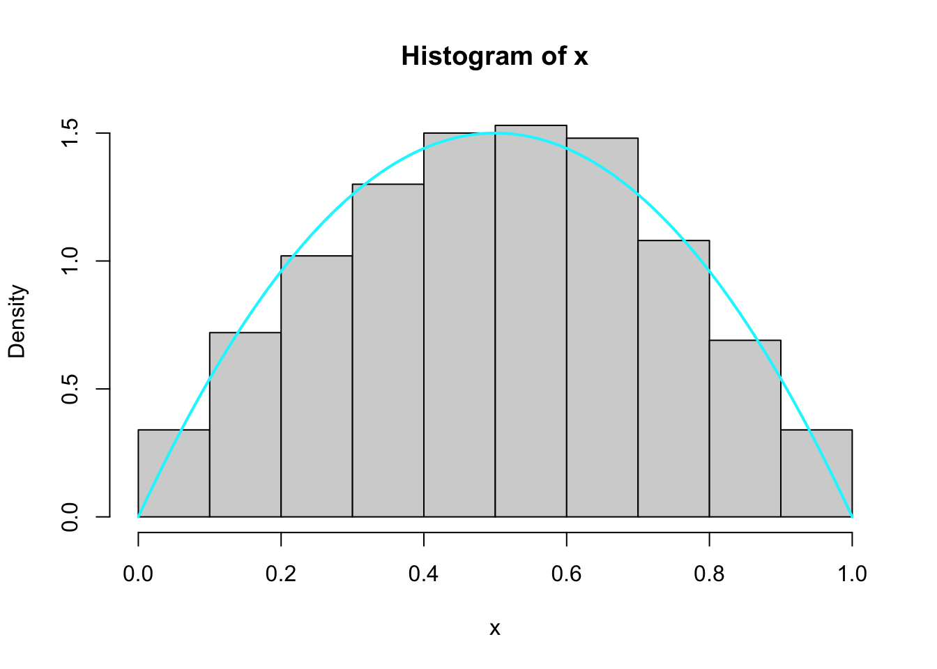

niter

::: {.cell-output .cell-output-stdout}

[1] 1532

::: :::

Compare Empirical and Theoretical Quantiles

\[ \text{se}(x_q) = \sqrt{\frac{p(1-p)}{n f^2(x_q)}} \]

Agreement between 1 and 2 SE is considered good:

p <- seq(.1, .9, .1)
samples <- quantile(x, p)
theoretical <- qbeta(p, 2, 2)
se <- sqrt(p * (1 - p) / n) * dbeta(theoretical, 2, 2)

diff <- samples - theoretical
diff <- diff / se
# plot table
cbind(samples, theoretical, diff)

      samples theoretical        diff
10% 0.1944411   0.1958001 -0.15162513
20% 0.2905545   0.2871407  0.21974679
30% 0.3742096   0.3632575  0.54457511
40% 0.4435312   0.4329311  0.46451623
50% 0.5107799   0.5000000  0.45451925
60% 0.5721829   0.5670689  0.22410331
70% 0.6347660   0.6367425 -0.09827994
80% 0.7093491   0.7128593 -0.22595231
90% 0.8038251   0.8041999 -0.04181931

Transformation Method

Relationship between common distributions:

• \(Z \sim N(0,1)\) then \(Z^2 \sim \chi^2_1\)

• \(U \sim \chi^2_m\) and \(V \sim \chi^2_n\) independent then \(F = \frac{U/m}{V/n} \sim F_{mn}\)

• \(T\) distribution:

  • \(U \sim \text{Gamma}(r, \lambda)\) and \(V \sim \text{Gamma}(s, \lambda)\) then \(X = \frac{U}{U+V} \sim \text{Beta}(r,s)\)

Example: simulate Beta from Gammas - Relationship does not depend on \(\lambda\). - Generate Beta(3,2):

n <- 1000
beta <- 2
alpha <- 3
u <- rgamma(n, shape = alpha, rate = 1)
v <- rgamma(n, shape = beta, rate = 1)
x <- u / (u + v)

p <- seq(.1, .9, .1)
samples <- quantile(x, p)
theoretical <- qbeta(p, alpha, beta)
plot(samples, theoretical, las = 1, pch = 21, bg = "red")
abline(0, 1, lwd = 2, col = "lightblue")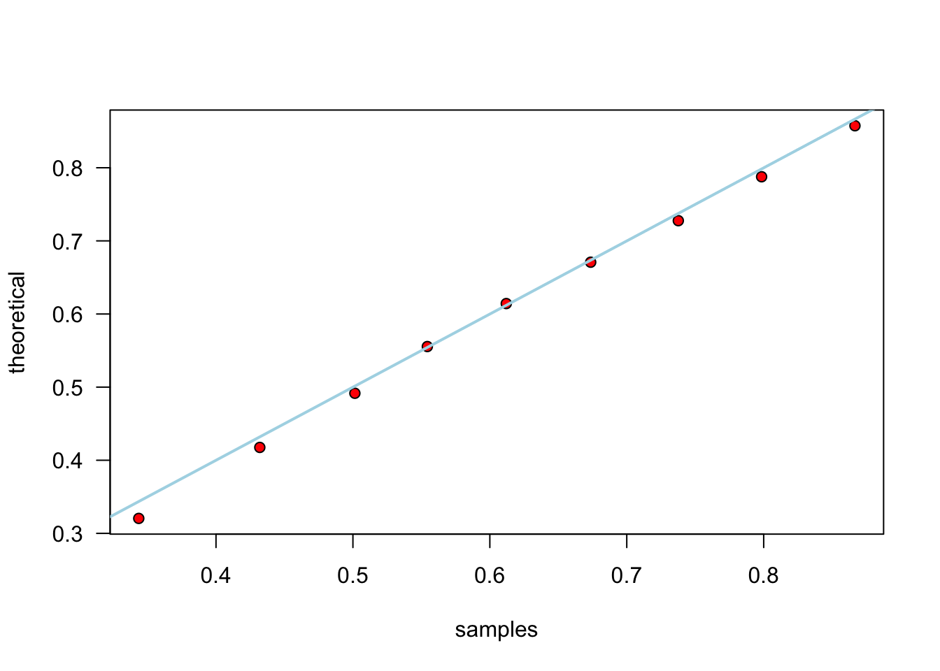

Sums and Mixtures

Convolution

• \(X_1, \ldots, X_n\) i.i.d.
• \(S = X_1 + X_2 + \ldots + X_n\)
• \(f_S\) is called the \(n\)-fold convolution of \(f_X\).
• Generate \(S \sim f_S\):
  • Generate \(X_1, X_2, \ldots, X_n\)
  • Set \(S = X_1 + X_2 + \ldots + X_n\)

Examples:

• \(\chi^2_r = \sum \chi^2_1\)
• \(\text{Gamma}(r, \lambda) = \sum \text{Exp}(\lambda)\)
• \(\text{Bin}(n, p) = \sum \text{Bin}(1, p)\)

Example: generate \(n\) \(\chi^2_{v}\):

n <- 1000
v <- 10
mat <- matrix(rnorm(n * v), n, v)
x <- rowSums(mat^2)
hist(x, prob = TRUE)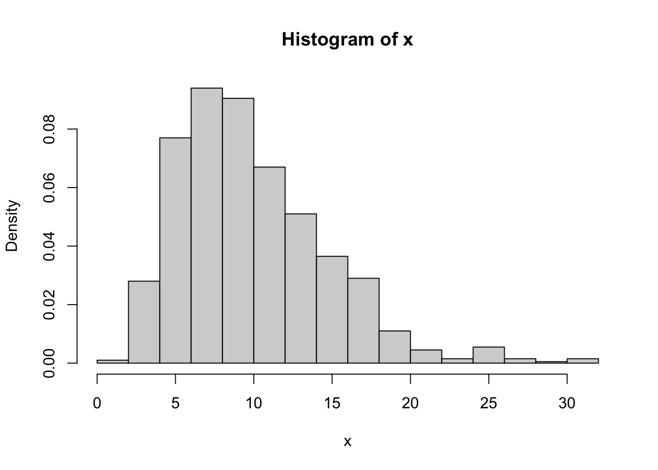

Compare theoretical and empirical quantiles:

p <- seq(.01, .99, .01)
samples <- quantile(x, p)
theoretical <- qchisq(p, v)
plot(samples, theoretical, las = 1, pch = 21, bg = "red")
abline(0, 1, lwd = 2, col = "lightblue")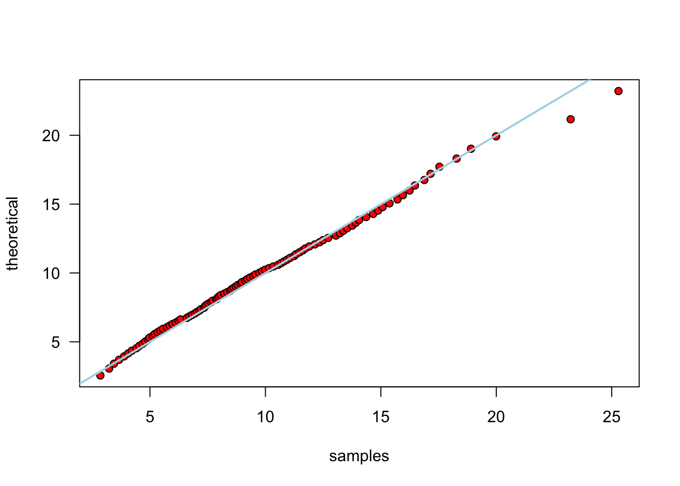

Convolutions of Poisson

• \(X_1 \sim \text{Poi}(\lambda_1)\), \(X_2 \sim \text{Poi}(\lambda_2)\)
• \(S = X_1 + X_2 \sim \text{Poi}(\lambda_1 + \lambda_2)\)

We show this using a transformation method:

• \(X = (X_1, X_2)\) in \(\mathbb{N}^2\)
• \(Y_1 = S = X_1 + X_2\), \(Y_2 = X_2\)
• \(X_1 = Y_1 - Y_2\), \(X_2 = Y_2\)
• Domain \(Y_1 \in \mathbb{N}\), \(Y_2 \leq Y_1\) \[ \frac{dx}{dy} = \begin{pmatrix} 1 & -1 \\ 0 & 1 \end{pmatrix} \]
  • Determinant = 1
  • \(f_X(x) = f_{P_1} \cdot f_{P_2} = e^{-\lambda_1} \frac{\lambda_1^{x_1}}{x_1!} \cdot e^{-\lambda_2} \frac{\lambda_2^{x_2}}{x_2!}\)
  • \(f_Y(y) = \text{Poi}(\lambda_1 + \lambda_2) \cdot \text{Bin}_{y_2}(y_1, \frac{\lambda_1}{\lambda_1 + \lambda_2})\)
  • Marginalize: \[ f_{Y_1}(y_1) = \text{Poi}(\lambda_1 + \lambda_2) \sum_{y_2=0}^{y_1} \text{Bin}_{y_2}(y_1, \frac{\lambda_1}{\lambda_1 + \lambda_2}) \] \[ f_{Y_1} = \text{Poi}(\lambda_1 + \lambda_2) \]

Mixtures

• \(X \sim f = \sum \pi f_i\) for some sequence of independent variables \(X_1, X_2, \ldots, X_n\) that may be infinite.
• Mixing weights \(\pi \geq 0\), \(\sum \pi = 1\)

Continuous: \[ X \sim f = \int_{-\infty}^{\infty} f_{X|Y} f_Y dy \] - \(f_{X|Y}\) family of distributions indexed by \(y\) weighted by \(f_Y\).

• Convolution vs. Mixture:
  • Convolution is a sum of i.i.d. random variables.
  • Mixture is a sum of densities weighted by a mixing distribution.

Example: Mixture of normals - \(f_X = \frac{1}{2} N(0,1) + \frac{1}{2} N(2,1)\)

Algorithm:

• Generate an integer \(k\) in \(\{1,2\}\) with \(P(k = 1) = \frac{1}{2}\).
• If \(k = 1\), generate \(X \sim N(0,1)\).
• If \(k = 2\), generate \(X \sim N(2,1)\).

Implementation:

n <- 1000
k <- sample(1:2, n, replace = TRUE, prob = c(1 / 2, 1 / 2))
x <- numeric(n)
for (i in 1:n) {
  if (k[i] == 1) {
    x[i] <- rnorm(1)
  } else {
    x[i] <- rnorm(1, 2, 1)
  }
}
hist(x, prob = TRUE)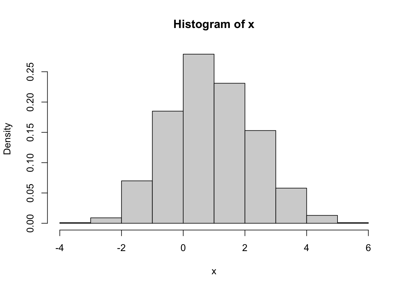

Example: Mixture of gammas

• \(f_X = \sum_{i=1}^{5} \pi_i f_{X_i}\) where \(X_i \sim \text{Gamma}(3, 1/i)\), \(\pi_i = \frac{i}{15}\)

Mean of \(f_{X_i}\): \(3i\)

Mean of \(f_X\): \[ \sum_{i=1}^{5} \frac{i}{15} \cdot 3i = 11 \]

::: {.cell}

mean <- sum((1:5) * (1:5) / 5)
mean

::: {.cell-output .cell-output-stdout}

[1] 11

::: :::

Generate 1000 samples:

n <- 1000
pi <- 1:5 / 15
rates <- 1 / (1:5)
mat <- matrix(rgamma(n * 5, shape = 3, rate = 1 / (1:5)), n, 5)
x <- rowSums(mat * pi)
plot(density(x), ylim = c(0, 0.5), col = "black")
# overlay plots of the 5 mixture densities of the gammas
y <- seq(0, max(x), length.out = 1000)
for (i in 1:5) {
  lines(y, dgamma(y, shape = 3, rate = rates[i]), col = i, lwd = 2)
}

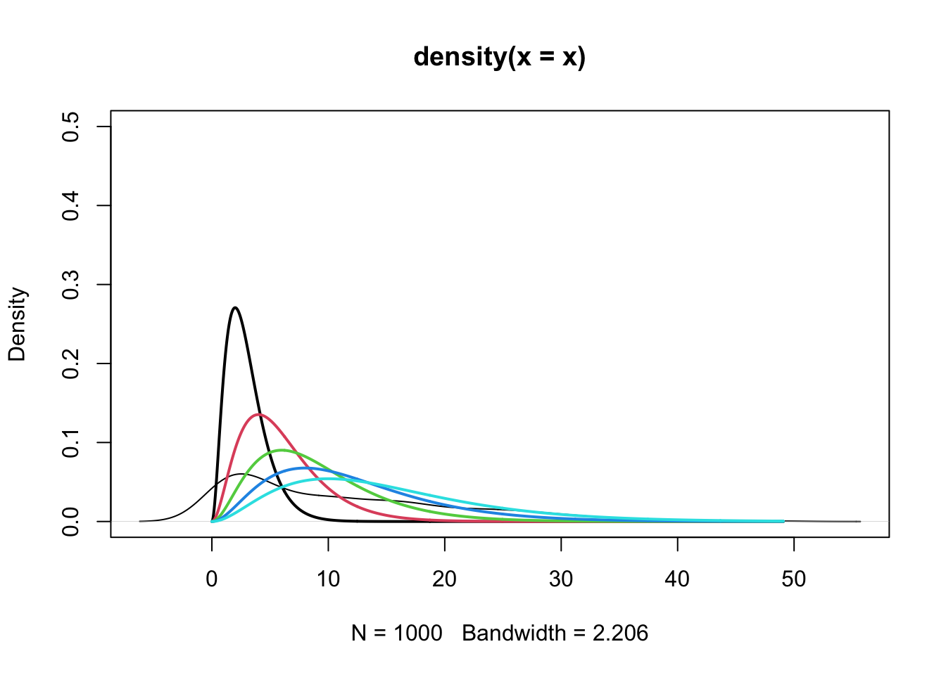
mean_x <- mean(x)
mean_x

[1] 11.1973

Negative binomial is a Poisson-Gamma mixture:

• \(X \sim f(x|\lambda) = \text{Poisson}(\lambda)\)
• Normally Poisson has only one parameter.
• To model overdispersion, we can use a gamma distribution: \[ \lambda \sim \text{Gamma}(r, \beta) \] \[ X \sim f_X = \int_{0}^{\infty} \text{Poisson}(x|\lambda) \text{Gamma}(\lambda|r,\beta) d\lambda \] \[ f_X = \text{NegBin}(r, p = \frac{\beta}{\beta + 1}) \]

Discrete distribution: number of failures before \(r\) successes in a sequence of independent Bernoulli trials with success probability \(p\): \[ f_X = \binom{x+r-1}{x} p^r (1-p)^x \]

::: {.cell}

set.seed(100)
n <- 1000
r <- 4
beta <- 3
lambda <- rgamma(n, r, beta)
x <- rpois(n, lambda)
barplot(table(x) / n,
col = "tomato",
las = 1, ylab = "simulated pdf", xlab = "x"
)

::: {.cell-output-display} ::: :::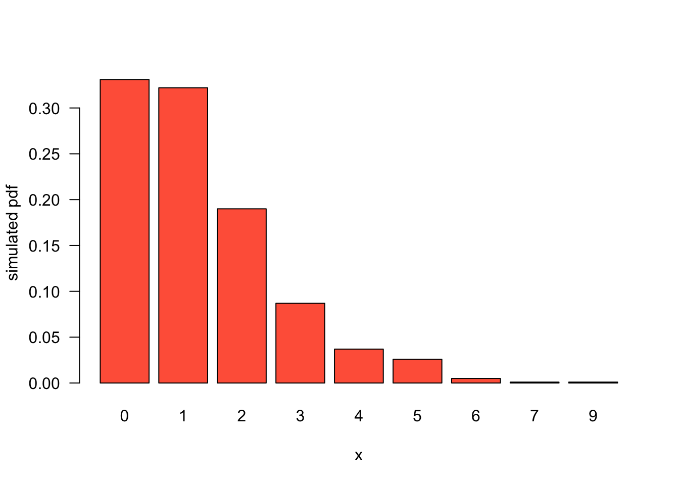

Comparing the theoretical and empirical quantiles for discrete distributions does not work well because the theoretical quantiles are not unique. - Standard error of ECDF is a better way to compare: \[ \text{se}(F_x) = \sqrt{\frac{F_n (1-F_n)}{n}} \]

::: {.cell}

set.seed(100)
sim <- table(x) / n

unique_x <- sort(unique(x))
truth <- dnbinom(unique_x, r, beta / (beta + 1))
diff <- sim - truth
two_se <- 2 * sqrt(truth * (1 - truth) / n)

tab <- round(rbind(unique_x, sim, truth, diff, two_se), 3)
# print table nicely
tab

::: {.cell-output .cell-output-stdout}

             0     1      2      3      4     5      6      7     9
unique_x 0.000 1.000  2.000  3.000  4.000 5.000  6.000  7.000 9.000
sim      0.331 0.322  0.190  0.087  0.037 0.026  0.005  0.001 0.001
truth    0.316 0.316  0.198  0.099  0.043 0.017  0.006  0.002 0.000
diff     0.015 0.006 -0.008 -0.012 -0.006 0.009 -0.001 -0.001 0.001
two_se   0.029 0.029  0.025  0.019  0.013 0.008  0.005  0.003 0.001

::: :::

Multivariate Distributions:

• mvnorm in the MASS package

• rmvnorm in the mvtnorm package

• We can generate them from \(N(0,1)\).

  \[ X \sim N(\mu, \sigma^2) \] \[ X = \sigma Z + \mu \]

Proof it works by the density transformation formula:

• \(Z \sim N(0,1)\) then: \[ f_Z(z) = \frac{1}{\sqrt{2\pi}} e^{- \frac{1}{2} z^2} \]
• \(X = \frac{X - \mu}{\sigma}\), \(\frac{dz}{dx} = \frac{1}{\sigma}\) \[ f_X(X) = f_Z \left(\frac{X - \mu}{\sigma}\right) \left|\frac{dz}{dx}\right| = \frac{1}{\sqrt{2\pi}\sigma} e^{- \frac{1}{2} \left(\frac{X - \mu}{\sigma}\right)^2} = N(\mu, \sigma^2) \]

We extend this scale and shift result to the multivariate case.

Multivariate normal generator:

• \(Y\) from \(N(\mu, \epsilon)\)

Algorithm:

• Cholesky decomposition of \(\epsilon = Q'Q\) in R using the chol function:
  • \(Z = (Z_1, Z_2, \ldots, Z_p) \sim N(0,I)\) \[ Y = \mu + Q'Z \]
    • \(E[Y] = Q'E[Z] + \mu = 0 + \mu = \mu\)
    • \(\text{Var}[Y] = Q'IQ = QQ' = \epsilon\)
    • \(Y\) is normally distributed with mean \(\mu\) and covariance \(\epsilon\).

n <- 100000
p <- 3
mat <- matrix(rnorm(n * p), n, p)
epsilon <- matrix(rnorm(p * p), p, p)
epsilon <- t(epsilon) %*% epsilon
Q <- chol(epsilon)
m <- rnorm(p)
mu <- matrix(m, n, p, byrow = TRUE)

x <- mat %*% Q + mu
# shape
# x[1,] # corresponds to a rv with mean mu and covariance epsilon the first one
mean <- apply(x, 2, mean)
round(cov(x), 1)

     [,1] [,2] [,3]
[1,]  5.9  1.6 -2.7
[2,]  1.6  2.5  0.4
[3,] -2.7  0.4  2.4

round(epsilon, 1)

     [,1] [,2] [,3]
[1,]  5.9  1.7 -2.7
[2,]  1.7  2.6  0.4
[3,] -2.7  0.4  2.5

Wishart Distribution

The chi-square is often used to model sample variances \(s^2\):

• From elementary statistics: \[ \frac{(n-1)s^2}{\sigma^2} \sim \chi^2_{n-1} \]
• The chi-square distribution with \(d_f\) degrees of freedom, \(\chi^2_{d_f}\), is a special case of the gamma distribution with shape parameter \(\frac{d_f}{2}\) and rate parameter \(\frac{1}{2}\), which means it has density: \[ f(x) = \frac{x^{\frac{d_f}{2}-1}}{2^{\frac{d_f}{2}} \Gamma(\frac{d_f}{2})} e^{-x/2}, \quad x \geq 0 \]

The Wishart distribution extends this to distributions for positive definite symmetric sample covariance matrices \(X \in \mathbb{R}^{p \times p}\) estimating a multivariate Normal variance \(V\):

\[ f(X) = \frac{|X|^{\frac{n-p-1}{2}}}{2^{\frac{np}{2}} |V|^{\frac{n}{2}} \Gamma_p\left(\frac{n}{2}\right)} \exp\left(-\frac{\text{tr}(V^{-1}X)}{2}\right) \] with \(\Gamma_p(\cdot)\) the multivariate gamma function and \(|\cdot|\) the determinant. This density is called \(W_p(V, n)\).

Generating from the Wishart distribution:

• Recall from earlier:

  • If \(Z_1, \ldots, Z_v\) are iid \(N(0,1)\) random variables, then \(V = Z_1^2 + \ldots + Z_v^2 \sim \chi^2_v\).

Generalize to:

• \(Z_1, \ldots, Z_n \in \mathbb{R}^p\) iid \(N_p(0, V) \rightarrow W = \sum_{i=1}^n Z_i Z_i' \sim W_p(V, n)\).

Excerise 3

Function to Generate from the F Distribution

n_samples <- 1000
m <- 10
n <- 10

# Function to generate F distribution samples
generate_f <- function(n_samples, m, n) {
  # Generate chi-squared random variables with m degrees of freedom
  chim <- rchisq(n_samples, m)
  chim <- chim / m
  # Generate chi-squared random variables with n degrees of freedom
  chin <- rchisq(n_samples, n)
  chin <- chin / n
  # F distribution is the ratio of two scaled chi-squared variables
  f <- chim / chin
  return(f)
}

# Generate F distribution samples
f <- generate_f(n_samples, m, n)
# Plot histogram of the F distribution samples
hist(f, col = "blue", main = "Histogram of F distribution", xlab = "Value", ylab = "Frequency")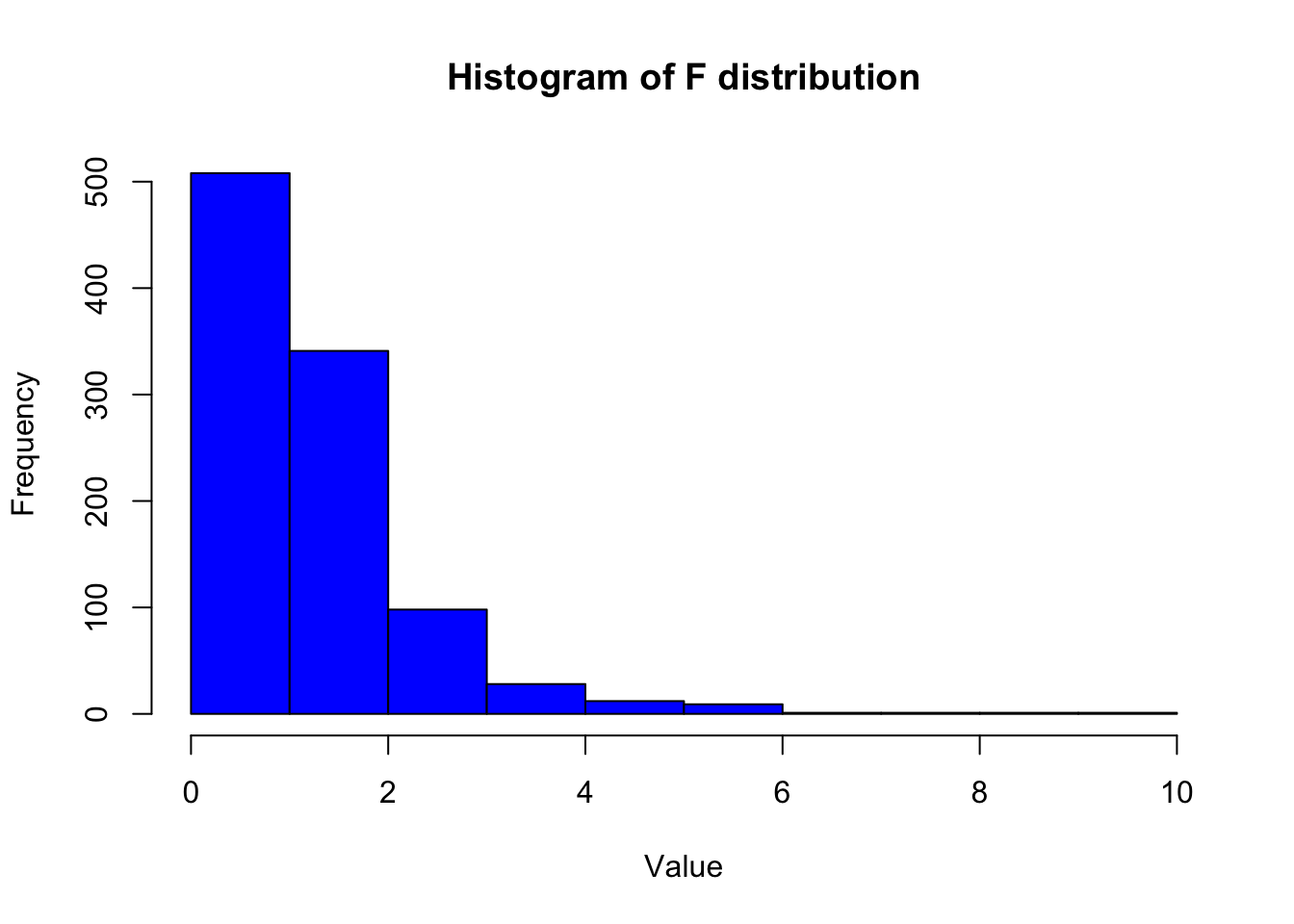

Plot a histogram of the random variables and a quantile plot against the theoretical (F) quantiles using qf and ppoints

# Generate theoretical quantiles from the F distribution
theoretical_quantiles <- qf(ppoints(n_samples), m, n)
# QQ plot of the theoretical quantiles against the generated samples
qqplot(theoretical_quantiles, f, main = "QQ Plot of F distribution", xlab = "Theoretical Quantiles", ylab = "Sample Quantiles")
# Add a QQ line
qqline(f, distribution = function(p) qf(p, m, n))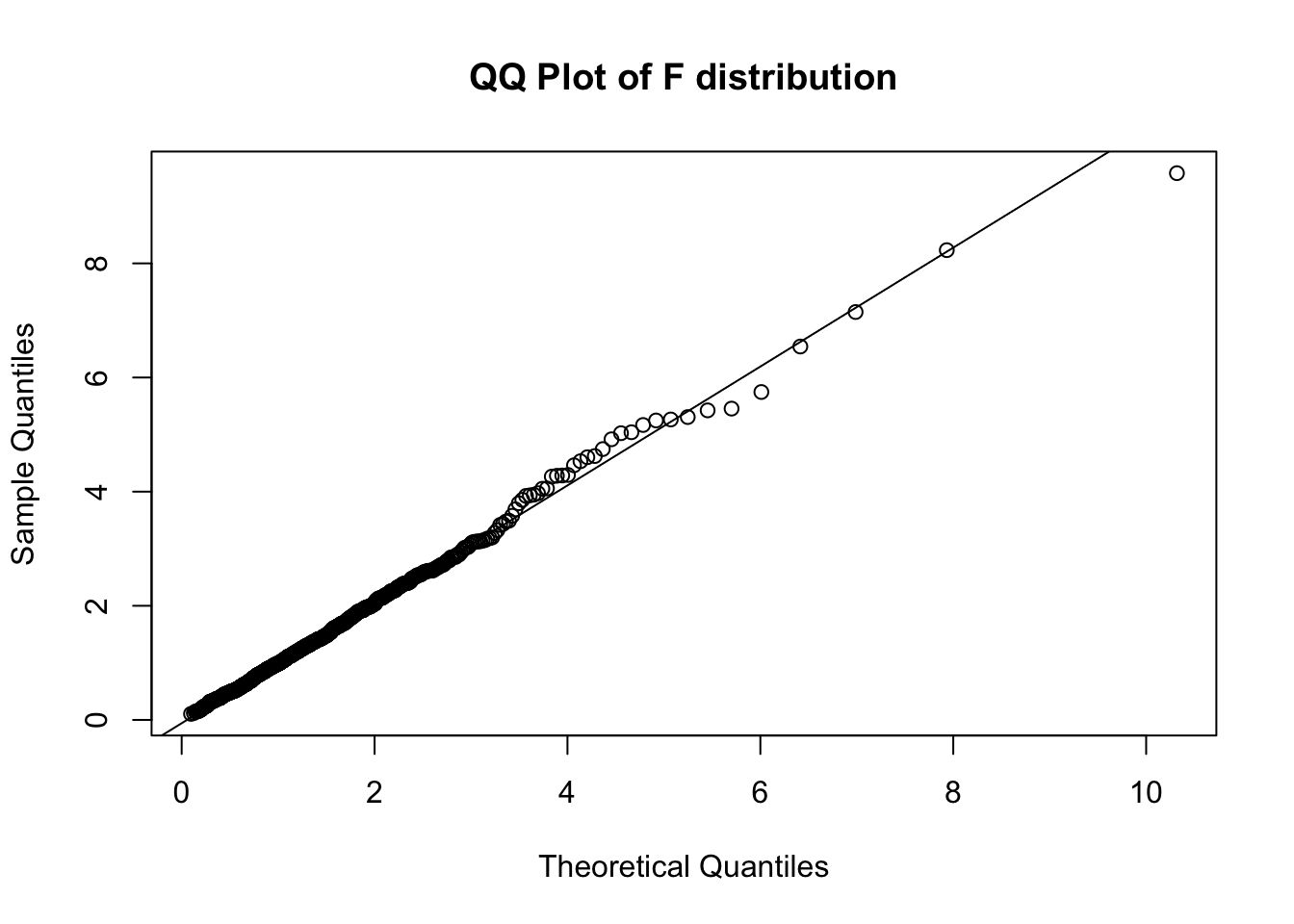

Generate from Normal-Gamma Mixture for a (t_4) Distribution

# Install invgamma package if not already installed
# install.packages('invgamma')
library(invgamma)

n <- 1000
v <- 4

# Generate inverse gamma random variables
vars <- rinvgamma(n, v/2, v/2)
# Generate normal random variables with variances from the inverse gamma distribution
x <- rnorm(n, 0, sqrt(vars))

# Plot histogram of the t4 distribution samples
hist(x, col = "green", main = "Histogram of t4 distribution", xlab = "Value", ylab = "Frequency")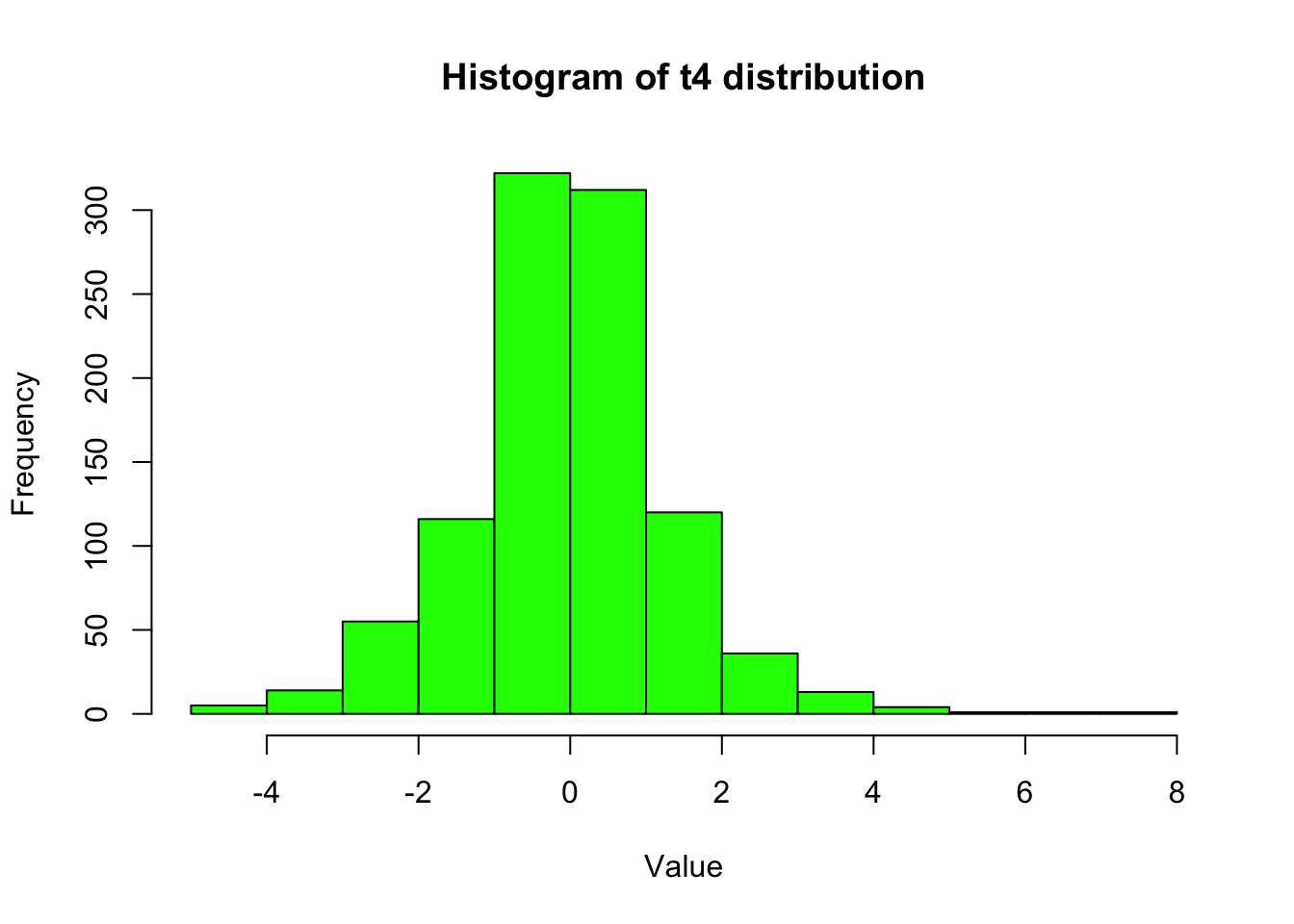

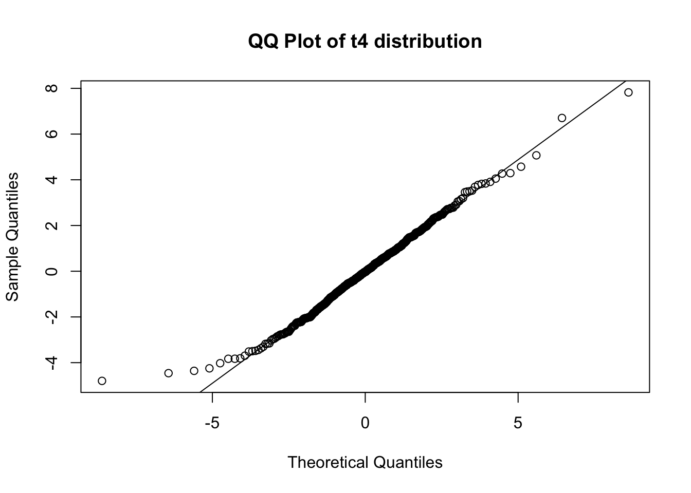
Plot a QQ Plot

# QQ plot of the generated t4 distribution samples against the theoretical t4 quantiles
qqplot(qt(ppoints(n), v), x, main = "QQ Plot of t4 distribution", xlab = "Theoretical Quantiles", ylab = "Sample Quantiles")
# Add a QQ line
qqline(x, distribution = function(p) qt(p, v))