detach(iris)# Create matrices and explore their propertiesy <-matrix(1:6, 3)x <-array(1:9, c(1, 3, 3))print(class(x))
[1] "array"
print(dim(x))
[1] 1 3 3
# Create and explore a named listnamed_list <-list(x =1, y ="c")print(named_list)
$x
[1] 1

$y
[1] "c"
print(named_list[[1]]) # Access by index
[1] 1
print(named_list$x) # Access by name
[1] 1
print(str(named_list)) # Structure of the list
List of 2
 $ x: num 1
 $ y: chr "c"
NULL
# Perform a t-test and explore the resultstat <-t.test(rnorm(2, 1, sd =3))print(str(stat))
List of 10
 $ statistic  : Named num 0.188
  ..- attr(*, "names")= chr "t"
 $ parameter  : Named num 1
  ..- attr(*, "names")= chr "df"
 $ p.value    : num 0.882
 $ conf.int   : num [1:2] -35.7 36.8
  ..- attr(*, "conf.level")= num 0.95
 $ estimate   : Named num 0.537
  ..- attr(*, "names")= chr "mean of x"
 $ null.value : Named num 0
  ..- attr(*, "names")= chr "mean"
 $ stderr     : num 2.85
 $ alternative: chr "two.sided"
 $ method     : chr "One Sample t-test"
 $ data.name  : chr "rnorm(2, 1, sd = 3)"
 - attr(*, "class")= chr "htest"
NULL
print(summary(stat))
            Length Class  Mode
statistic   1      -none- numeric
parameter   1      -none- numeric
p.value     1      -none- numeric
conf.int    2      -none- numeric
estimate    1      -none- numeric
null.value  1      -none- numeric
stderr      1      -none- numeric
alternative 1      -none- character
method      1      -none- character
data.name   1      -none- character
print(stat)
    One Sample t-test

data:  rnorm(2, 1, sd = 3)
t = 0.18827, df = 1, p-value = 0.8815
alternative hypothesis: true mean is not equal to 0
95 percent confidence interval:
 -35.73128  36.80609
sample estimates:
mean of x
0.5374071
print(unlist(stat))
          statistic.t          parameter.df               p.value
  "0.188272736184213"                   "1"   "0.881528665093894"
            conf.int1             conf.int2    estimate.mean of x
   "-35.731275046196"    "36.8060891481264"   "0.537407050965217"
      null.value.mean                stderr           alternative
                  "0"    "2.85440718532607"           "two.sided"
               method             data.name
  "One Sample t-test" "rnorm(2, 1, sd = 3)"
print(unclass(stat))
$statistic
        t
0.1882727

$parameter
df
 1

$p.value
[1] 0.8815287

$conf.int
[1] -35.73128  36.80609
attr(,"conf.level")
[1] 0.95

$estimate
mean of x
0.5374071

$null.value
mean
   0

$stderr
[1] 2.854407

$alternative
[1] "two.sided"

$method
[1] "One Sample t-test"

$data.name
[1] "rnorm(2, 1, sd = 3)"
# Create a matrix with dimension namesmat <-matrix(1:4, 2)dimnames(mat) <-list(c("0", "1"), c("x", "y"))print(mat)
  x y
0 1 3
1 2 4
row.names(mat) <- letters[1:2]print(mat)
  x y
a 1 3
b 2 4
# Graphics# Attach iris dataset for direct column accessattach(iris)print(names(iris))
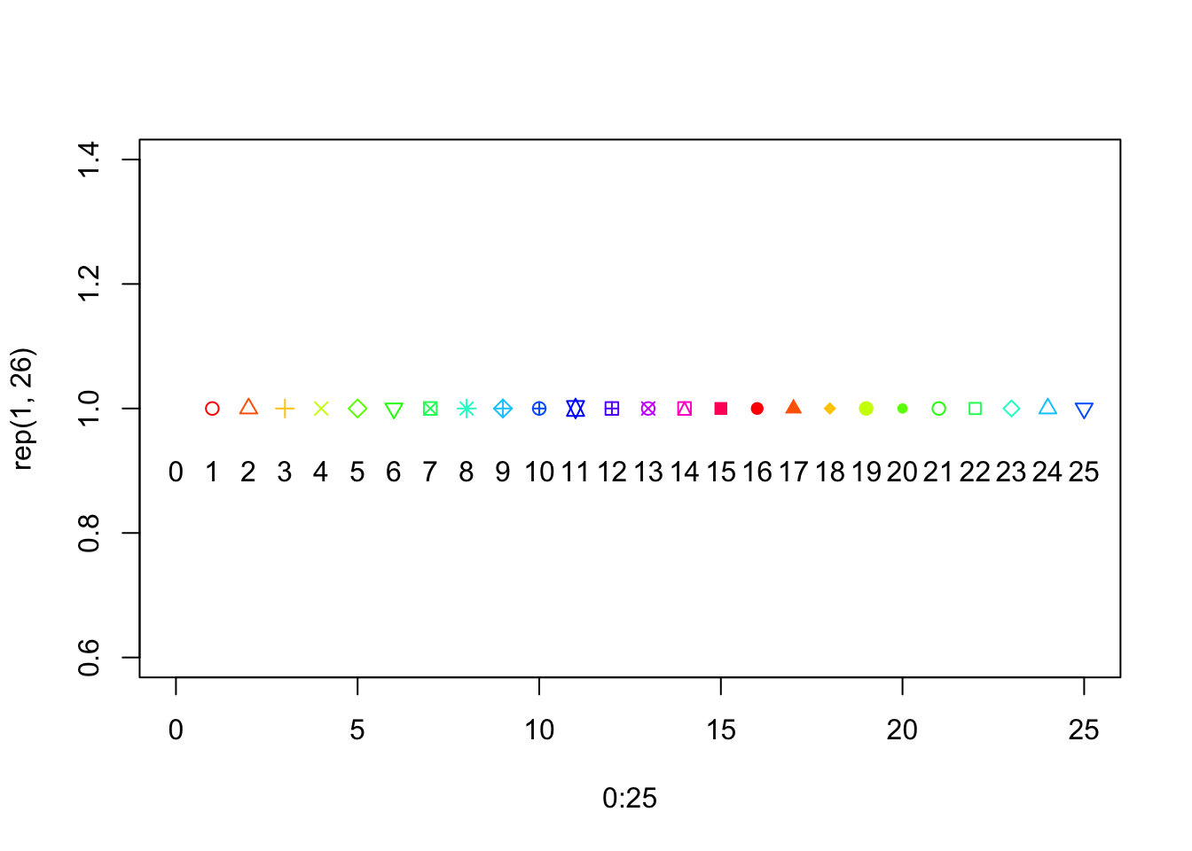
plot(0:25, rep(1, 26), pch =0:25, col =0:25)text(0:25, 0.9, 0:25)
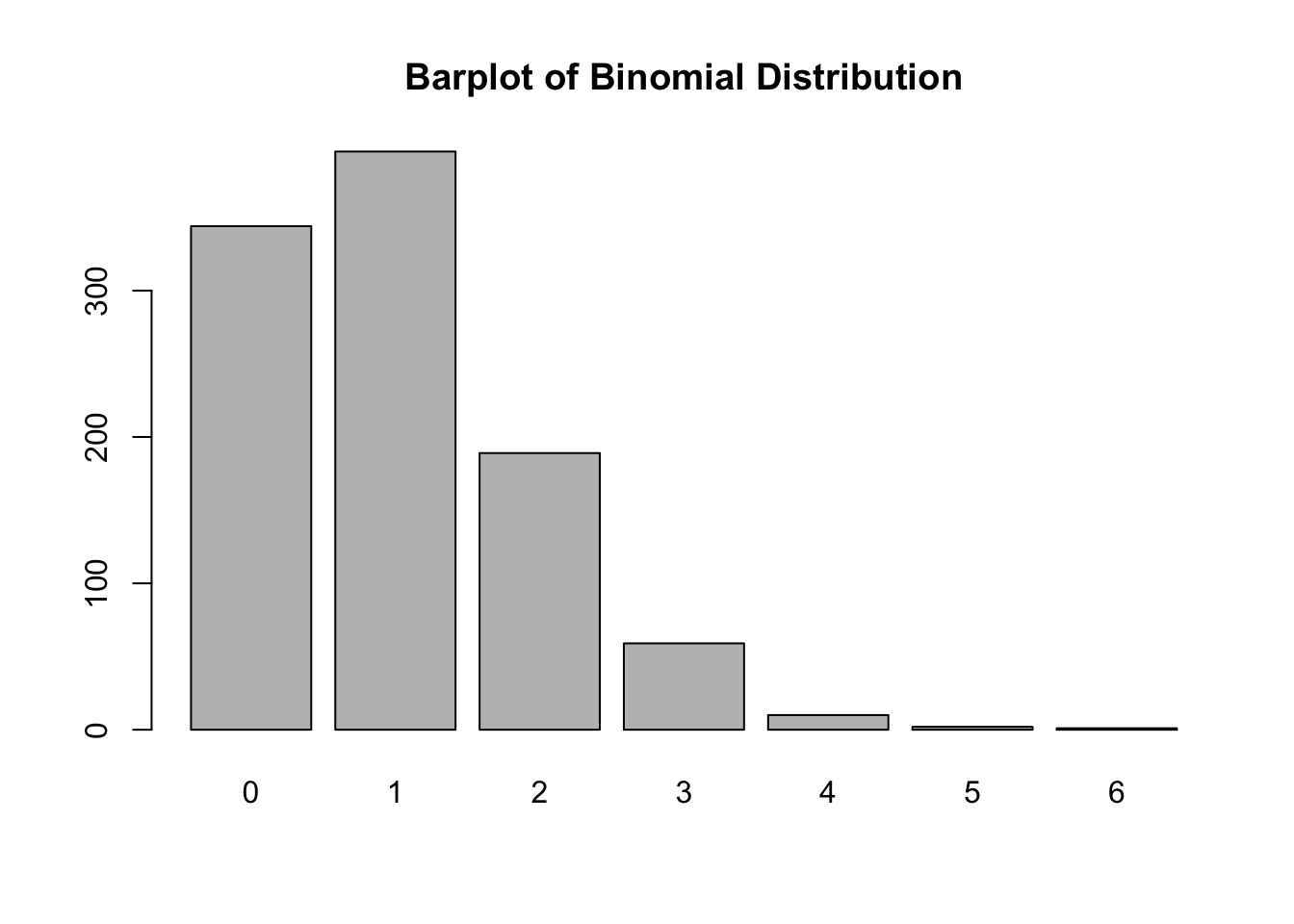
# Example of barplot using rbinomx <-rbinom(1000, 10, 0.1)barplot(table(x), main ="Barplot of Binomial Distribution")# ggplot2 exampleslibrary(ggplot2)
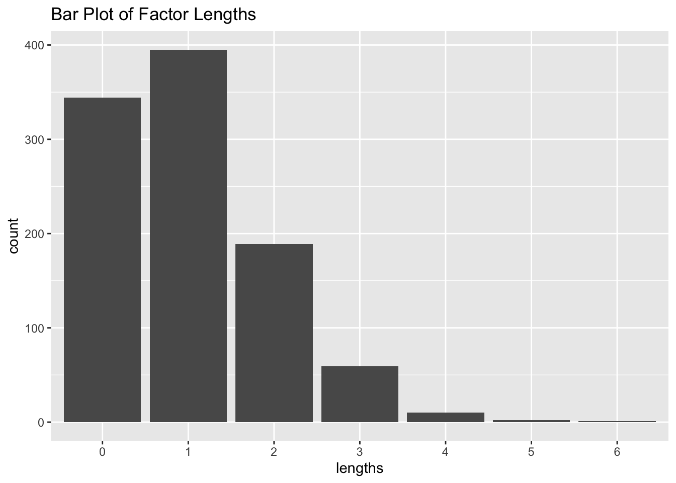
# Bar plotdf <-data.frame(lengths =factor(x))ggplot(df, aes(lengths)) +geom_bar() +ggtitle("Bar Plot of Factor Lengths")
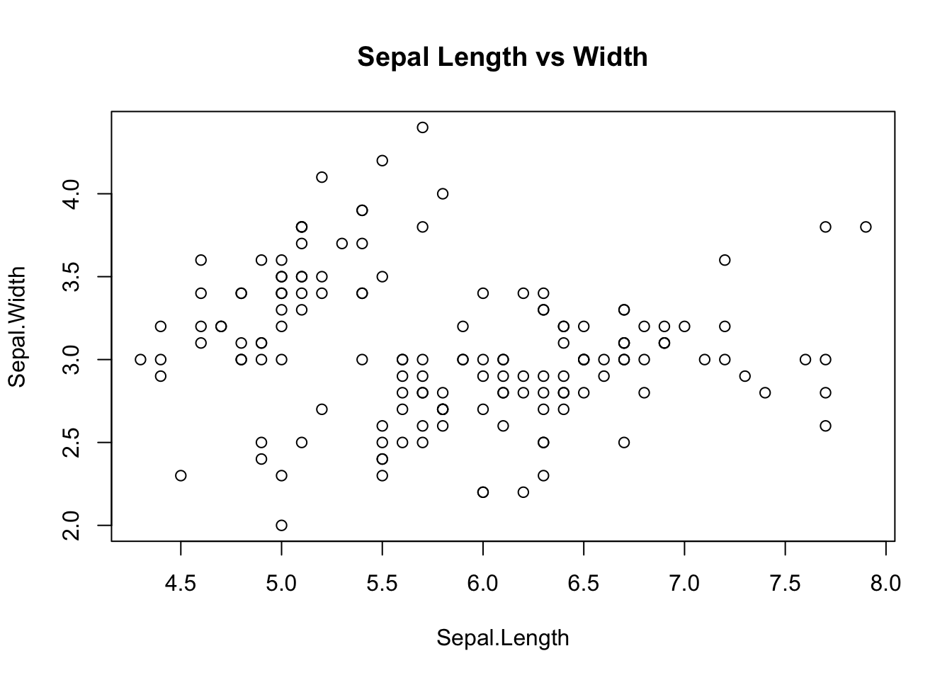
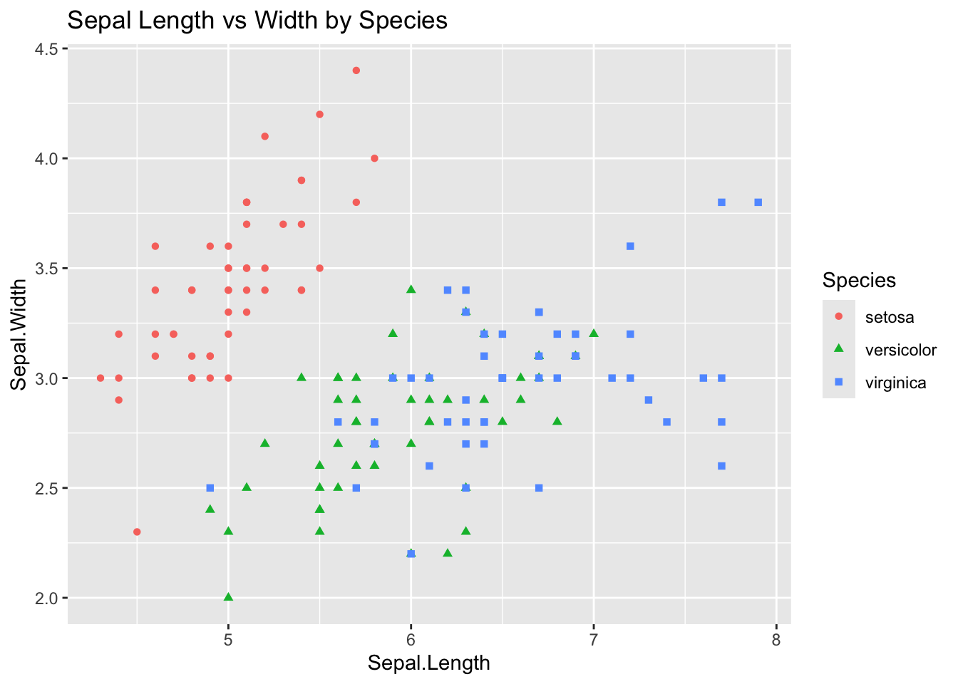
# Scatter plot of iris datasetggplot(data = iris, aes(x = Sepal.Length, y = Sepal.Width, color = Species, shape = Species)) +geom_point() +ggtitle("Sepal Length vs Width by Species")
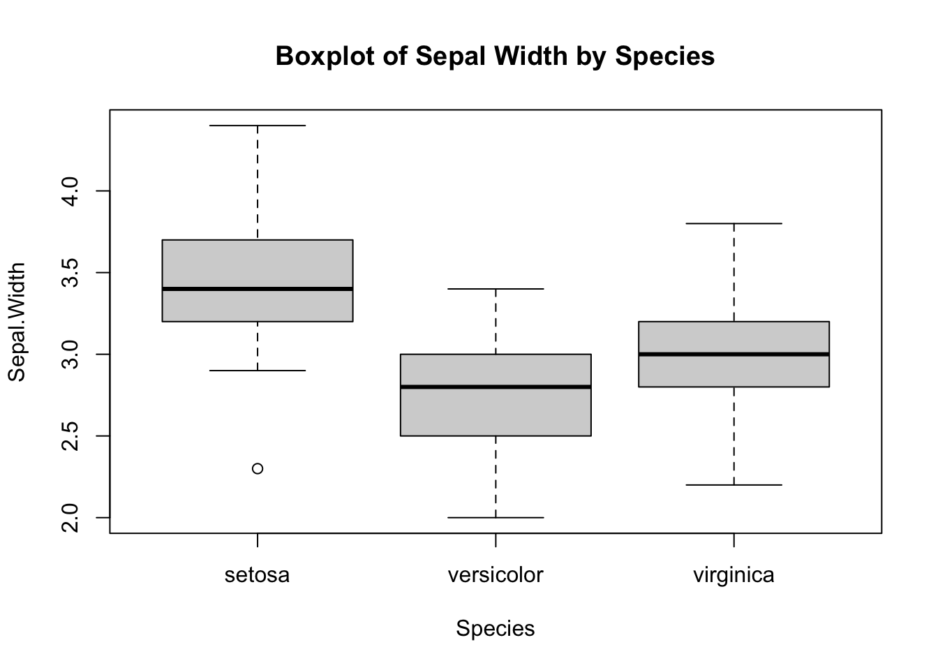
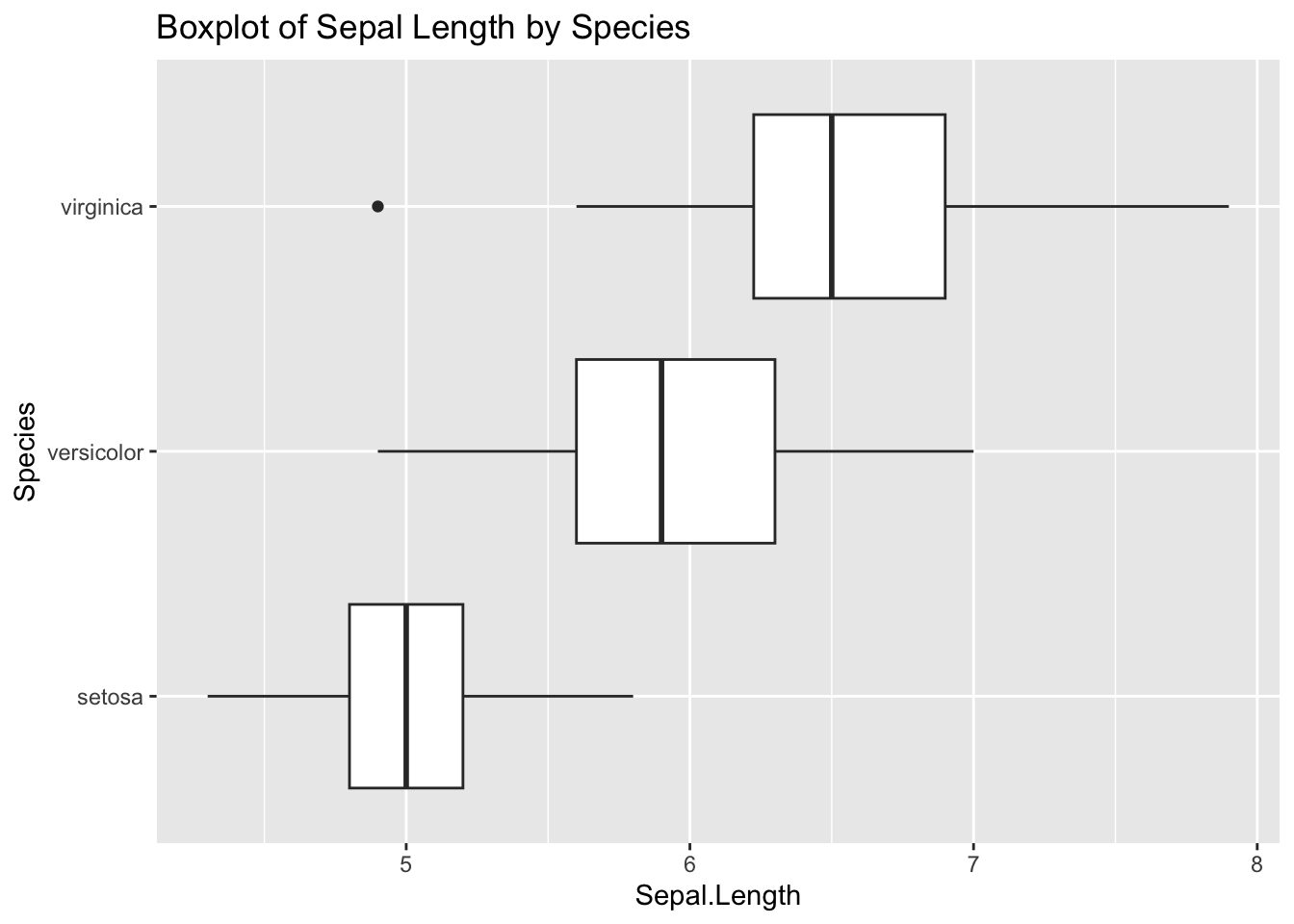
# Boxplot and Violin plot of Sepal Length by Speciesggplot(iris, aes(Species, Sepal.Length)) +geom_boxplot() +coord_flip() +ggtitle("Boxplot of Sepal Length by Species")
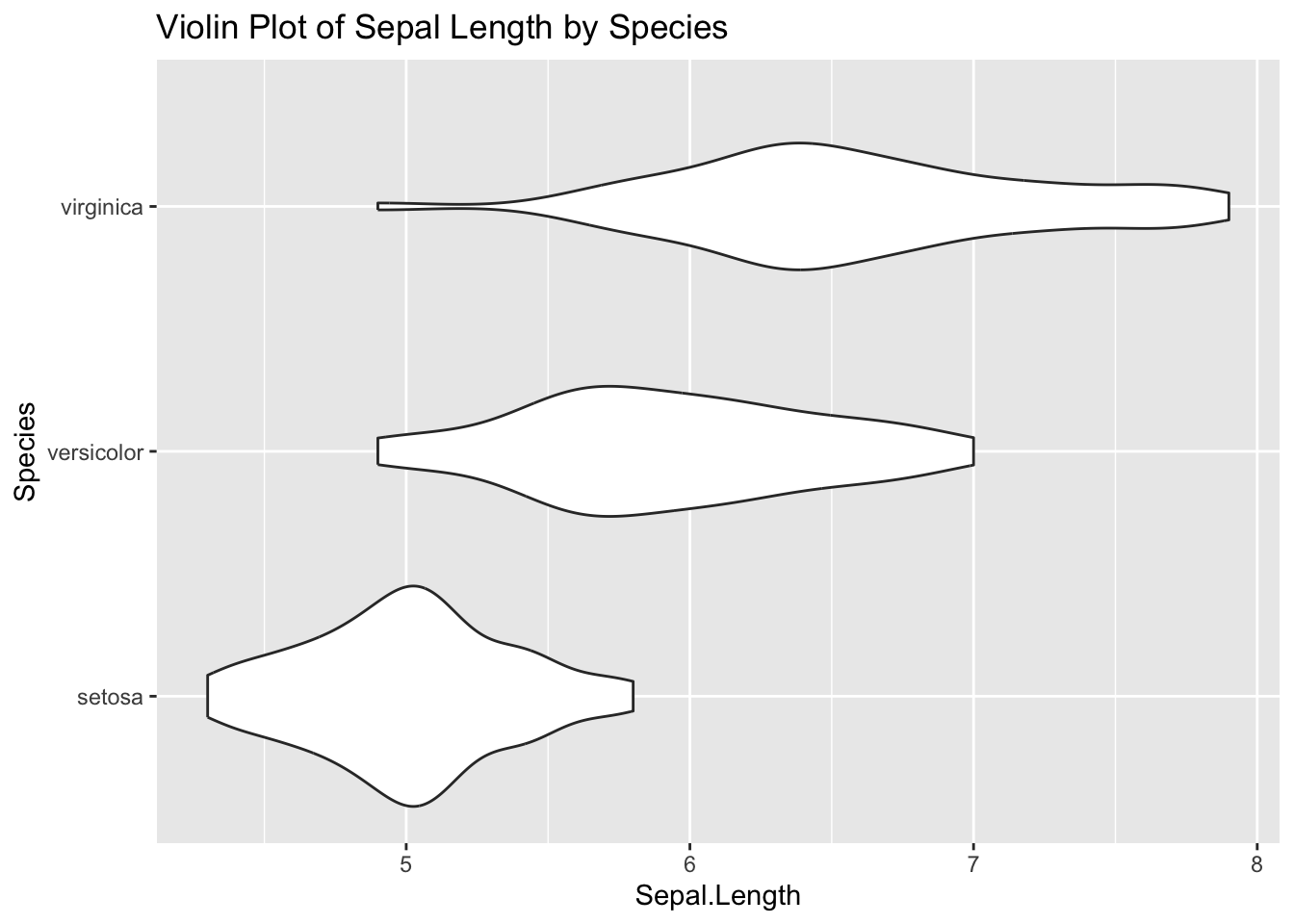
ggplot(iris, aes(Species, Sepal.Length)) +geom_violin() +coord_flip() +ggtitle("Violin Plot of Sepal Length by Species")
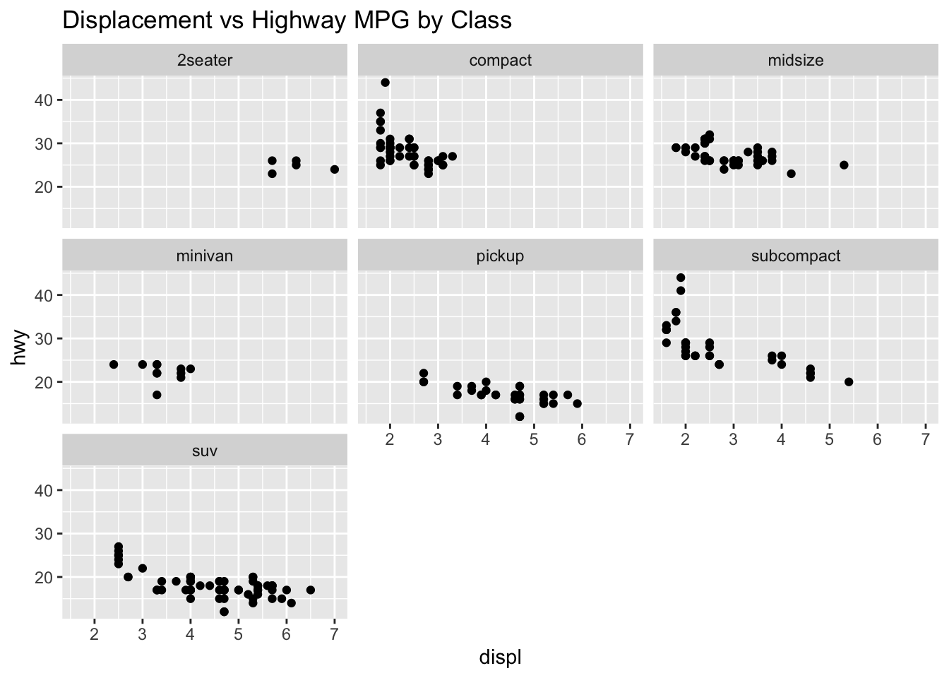
# Multiple plots using facet_wrapggplot(mpg, aes(displ, hwy)) +geom_point() +facet_wrap(~class) +ggtitle("Displacement vs Highway MPG by Class")
# Workspace managementprint(ls()) # List objects in workspace
[1] "df"         "mat"        "named_list" "squared"    "stat"
[6] "x"          "X"          "y"
rm("df") # Remove specific objectrm(list =ls()) # Remove all objects# Working directory managementprint(getwd())
\(X\) is multivariate normal with mean vector () and covariance matrix ().
\(Y\) is multivariate normal with mean \(A\mu + B\) and covariance \(A\Sigma A^T\).
Limit Theorems
Weak Law of Large Numbers
The sample mean converges in probability to the population mean. Let \(X_1, X_2, \ldots, X_n\) be i.i.d. random variables with \(E[|X_1|] < \infty\) and population mean \(\mu = E[X_1]\). Then:
\[ \bar{X} = \frac{1}{n} \sum_{i=1}^n X_i\]
converges in probability to \(\mu\) as \(n \to \infty\):
The sample mean converges almost surely to the population mean. Let \(X_1, X_2, \ldots, X_n\) be i.i.d. random variables with \(E[|X_1|] < \infty\) and population mean \(\mu = E[X_1]\). Then:
\[ \bar{X} = \frac{1}{n} \sum_{i=1}^n X_i\]
converges almost surely to \(\mu\) as \(n \to \infty\):
Algorithm: 1. Write down \(F_X(x)\). 2. Derive \(F_X^{-1}(u)\). 3. Generate \(U \sim U(0,1)\) and plug in \(F_X^{-1}(U)\).
Acceptance-Rejection Method
To sample from \(f(x)\) using proposal distribution \(g(x)\):
Find \(c > 0\) such that \(f(x) \leq c g(x)\) for all \(x\).
Sample \(y\) from \(g\) and \(u\) from \(U(0,1)\).
If \(u \leq \frac{f(y)}{c g(y)}\), accept \(x = y\).
Transformation Method
If \(Z \sim N(0, 1)\), then \(Z^2\) follows a chi-squared distribution with 1 degree of freedom.
Sum of \(Z^2\) (n times) is chi-squared with n degrees of freedom.
If \(U, V \sim \chi^2\) with \(m, n\) degrees of freedom, then \(\frac{U/m}{V/n}\) follows an F-distribution with \(m, n\) degrees of freedom.
If \(Z \sim N(0, 1)\) and \(V \sim \chi^2\) with \(n\) degrees of freedom, then \(\frac{Z}{\sqrt{V/n}}\) follows a t-distribution with \(n\) degrees of freedom.
If \(U, V\) are independent and uniform on (0,1), then: \[
z_1 = \sqrt{-2 \log U} \cos(2 \pi V), \quad z_2 = \sqrt{-2 \log U} \sin(2 \pi V)
\] are independent \(N(0,1)\).
Sums and Mixtures
If \(X_1, X_2\) are independent, then:
\(S = X_1 + X_2\) is the convolution of the distributions of \(X_1\) and \(X_2\).
Chi-squared with \(n\) degrees of freedom is the convolution of \(n\)\(N(0,1)\) squared variables.
Negative binomial is a convolution of \(n\) geometric distributions with parameter \(p\).
\(r\) independent exponential distributions with rate \(\lambda\) summed is gamma distributed with parameters \(r\) and \(\lambda\).
Row and column sums: - \(\text{apply}(X, 1, \sum)\) is row sums. - \(\text{apply}(X, 2, \sum)\) is column sums. - In Python: \(X.sum(axis=0)\) for column sums.
Mixtures
A discrete mixture: \(F_X = \sum \pi_i F_{X_i}\) where \(\pi_i \geq 0\) and \(\sum \pi_i = 1\).
A continuous mixture: \(F_X(x) = \int F_{X|Y}(x) f_Y(y) \, dy\).
Multivariate Normal Generation
To generate \(N(\mu, \Sigma)\) from \(N(0, I)\):
Let \(Z\) be \(N(0, I)\) (dimension \(d\)).
Factor \(\Sigma\) as \(\Sigma = C C^T\).
Then \(X = CZ + \mu \sim N(\mu, \Sigma)\).
Decomposition methods: - Eigen decomposition: \(\Sigma = V A V^T\). - SVD: \(\Sigma = U D V^T\). - Cholesky: \(\Sigma = L L^T\).
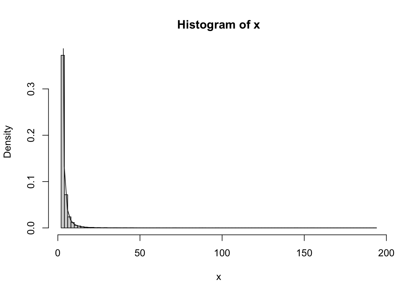
Pareto Distribution
The Pareto(a, b) distribution has CDF:
\[ F(x) = 1 - \left(\frac{b}{x}\right)^a, \quad x \geq b > 0, \; a > 0\]
Inverse transformation:
\[ F^{-1}(u) = b (1 - u)^{-1/a}\]
Simulation and histogram in R:
n =10000a =2b =2u =runif(n)x = b / (1- u)^(1/a)hist(x, prob =TRUE, breaks =100)curve(a * b^a / x^(a+1), add =TRUE)
Monte Carlo Integration and Variance Reduction
Monte Carlo Integration and Variance Reduction
To compute \(\int_0^1 g(x) \, dx\) where \(g\) is a function that is hard to integrate:
\[ E(g(X)) = \int g(x) f(x) \, dx\]
where \(f\) is the density of \(X\).
If \(X\) is uniform on ([0, 1]), then \(E(g(X)) = \int_0^1 g(x) \, dx\):
\[ \approx \frac{1}{n} \sum_{i=1}^n g(U_i)\]
where \(U_i\) are uniform on ([0, 1]).
This converges to the integral as \(n \to \infty\) with probability 1.
Generate antithetic variables to reduce variance. If \(m\) Monte Carlo replicates are required, generate \(m/2\) replicates \(Y_j = g(F_X^{-1}(U_j))\) and the remaining \(m/2\) replicates \(Y'_j = g(F_X^{-1}(1 - U_j))\), where \(U_j\) are i.i.d. uniform ([0,1]).
The antithetic estimator is: \[ \hat{\theta} = \frac{1}{m} \sum_{j=1}^{m/2} \left( Y_j + Y'_j \right)\]
Thus, \(nm/2\) rather than \(nm\) uniform variates are required, and the variance is reduced.
Control Variates
To reduce the variance in a Monte Carlo estimator of \(\theta = E[g(X)]\):
Suppose there is a function \(f\) such that \(\mu = E[f(X)]\) is known, and \(f(X)\) is correlated with \(g(X)\).
For any constant \(c\): \[ \hat{\theta}_c = g(X) + c(f(X) - \mu)\]
is minimized at: \[ c^* = -\frac{\text{Cov}(g(X), f(X))}{\text{Var}(f(X))}\]
with minimum variance: \[ \text{Var}(\hat{\theta}_{c^*}) = \text{Var}(g(X)) - \frac{\text{Cov}(g(X), f(X))^2}{\text{Var}(f(X))}\]
The random variable \(f(X)\) is called a control variate for the estimator \(g(X)\).
Antithetic variables are a special case of control variates. For any two unbiased estimators \(\hat{\theta}_1\) and \(\hat{\theta}_2\), the control variate estimator is: \[ \hat{\theta}_c = c \hat{\theta}_1 + (1 - c) \hat{\theta}_2\]
In the special case of antithetic variates, \(\hat{\theta}_1\) and \(\hat{\theta}_2\) are identically distributed and \(\text{Cor}(\hat{\theta}_1, \hat{\theta}_2) = -1\). The variance is minimized when \(c^* = \frac{1}{2}\), resulting in the antithetic estimator: \[ \hat{\theta}_{c^*} = \frac{\hat{\theta}_1 + \hat{\theta}_2}{2}\]
Importance Sampling
Suppose we want to estimate \(E[g(X)]\) where \(X\) is distributed according to \(f_X\).
Let \(g(x)\) be a function such that \(g(x) / f_X(x) > 0\).
For importance sampling to be effective, we want \(Y\) to be almost constant so that the variance is small. This means choosing \(f_X\) such that it is close to \(g(x)\) up to a constant factor.
Example in R
Simulating using importance sampling:
n =10000g =function(x) { x^2 }f_X =function(x) { dnorm(x, mean =0, sd =1) }X =rnorm(n)Y =g(X) /f_X(X)E_Y =mean(Y)E_Y