# Generate a sequence of numbers from 1 to 20 with a step of 2
print(seq(1, 20, 2))
[1] 1 3 5 7 9 11 13 15 17 19# Generate a sequence of numbers from 1 to 20 with a step of 2
print(seq(1, 20, 2)) [1] 1 3 5 7 9 11 13 15 17 19# Create a sequence of numbers from 1 to 20
1:20 [1] 1 2 3 4 5 6 7 8 9 10 11 12 13 14 15 16 17 18 19 20# Create a vector of numbers
x = c(1, 2, 3, 4, 5)
x[1] 1 2 3 4 5# Calculate the square root of 4
sqrt(4)[1] 2# Generate 5 random numbers from a uniform distribution
runif(5)[1] 0.78997690 0.52227519 0.67701569 0.28452173 0.07227832# Calculate the quantile function (inverse of CDF) for the normal distribution at 0.95
qnorm(0.95)[1] 1.644854# Get help on the pt function (t-distribution cumulative distribution function)
head(?pt)[1] "/Library/Frameworks/R.framework/Versions/4.3-arm64/Resources/library/stats/help/TDist"# Search for help on the term "pt"
# help.search("pt")# Calculate the cumulative probability for the t-distribution with 10 degrees of freedom at 1.96
pt(1.96, df = 10)[1] 0.9607819# Calculate the gamma density with shape = 1 and rate = 1
dgamma(1, shape = 1, rate = 1)[1] 0.3678794# Calculate the ranks of the numbers in the vector
rank(c(1, 3, 2, 4, 5, 5, 5))[1] 1 3 2 4 6 6 6# Sort the numbers in decreasing order
sort(c(5, 3, 2, 1, 4), decreasing = TRUE)[1] 5 4 3 2 1# Generate 100 random numbers from a normal distribution
x = rnorm(50)# Calculate the standard deviation of the generated numbers
x_sd = sd(x)
x_sd[1] 0.9701469# Calculate the correlation between x and -x
correlation = cor(x, -x)
correlation[1] -1# Create a table showing the number of positive and non-positive numbers in x
table(x > 0)
FALSE  TRUE
   25    25
# Handle missing values in a vector
z = c(1, 2, NA, 4, 5)
z[1] 1 2 NA 4 5# Check for missing values in z
is.na(z)[1] FALSE FALSE TRUE FALSE FALSE# {R}emove missing values from z
z[!is.na(z)][1] 1 2 4 5# Check if the density of the normal distribution at 0 equals 1/sqrt(2*pi)
dnorm(0) == 1/sqrt(2*pi)[1] TRUE# Check if the CDF of the normal distribution at 0 equals 0.5
pnorm(0) == 0.5[1] TRUE# Check if the quantile function of the normal distribution at 0 equals -Inf
qnorm(0) == -Inf[1] TRUE# Calculate the density of the normal distribution at 0 with mean = 2 and sd = 5
means = 2
sdev = 5
dnorm(0, mean = means, sd = sdev)[1] 0.07365403# Create a 3x2 matrix filled by column with numbers 1 to 6
mat = matrix(1:6, nrow = 3, ncol = 2)
mat [,1] [,2]
[1,] 1 4
[2,] 2 5
[3,] 3 6# Create a 3x2 matrix filled by row with numbers 1 to 6
mat = matrix(1:6, 3, byrow = TRUE)
mat [,1] [,2]
[1,] 1 2
[2,] 3 4
[3,] 5 6# Create a numeric vector of length 4
numeric(4)[1] 0 0 0 0# Create an integer vector of length 4
integer(4)[1] 0 0 0 0# {R}epeat the number 1, 4 times
rep(1, 4)[1] 1 1 1 1# Create a 2x3 matrix filled with zeros
mat = matrix(0, 2, 3)
mat [,1] [,2] [,3]
[1,] 0 0 0
[2,] 0 0 0# Access the first column of the matrix
mat[, 1][1] 0 0# Access the first row of the matrix
mat[1, ][1] 0 0 0# Access the element in the first row and first column
mat[1, 1][1] 0# Compute the square of the matrix by matrix multiplication
mat_sqvr = mat %*% t(mat)
mat_sqvr [,1] [,2]
[1,] 0 0
[2,] 0 0# Multiply two vectors element-wise
rep(1, 4) * rep(3, 4)[1] 3 3 3 3# Create a 3x3 matrix filled by column with numbers 1 to 9
mat = matrix(1:9, 3, 3)# Non sigular
mat = matrix(c(1, 2, 3, 4), 2, 2)
# Calculate the inverse of the matrix
solve(mat) [,1] [,2]
[1,] -2 1.5
[2,] 1 -0.5# Extract the diagonal elements of the matrix
diag(mat)[1] 1 4# Create a scatter plot
plot(1:10, seq(1, 20, 2))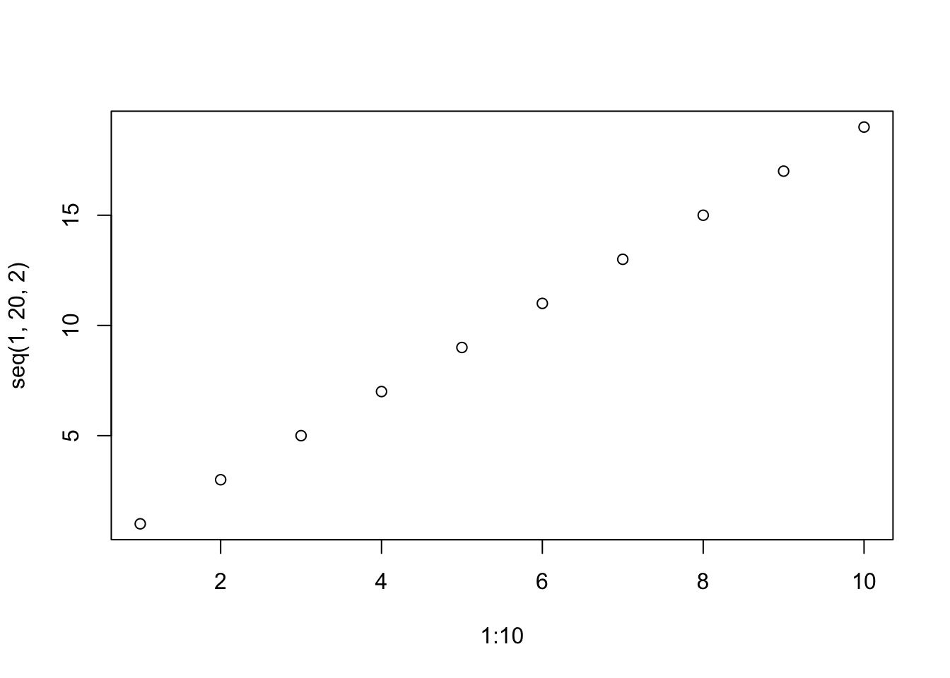
# Create a line plot with customizations
plot(1:10, seq(1, 20, 2), type = "l", col = "blue", lwd = 2, main = "Line Plot", xlab = "X-axis", ylab = "Y-axis")
abline(h = 10, col = "red", lwd = 6)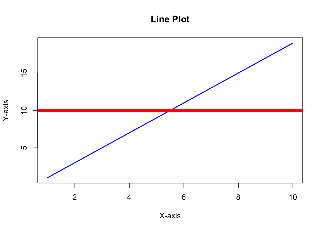
# Add a curve to the existing plot
# curve(x^2, from = -10, to = 10, col = "green", lwd = 2, lty = 1, add = TRUE)
# Create a histogram of 1000 random normal numbers
hist(rnorm(1000), col = "blue", main = "Histogram of 1000 random normal numbers", xlab = "Value", ylab = "Frequency")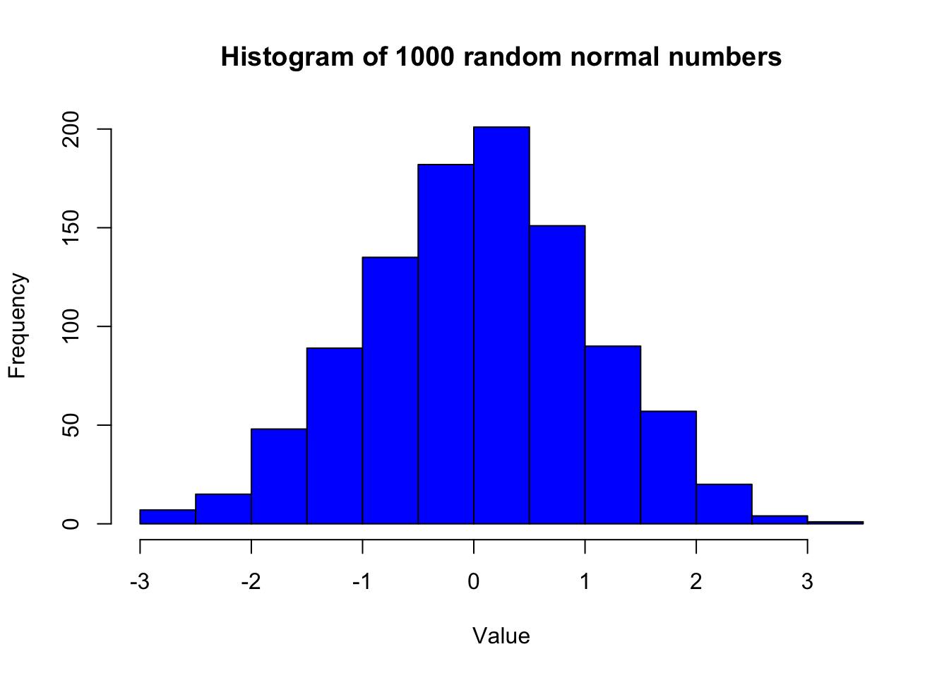
# Create a barplot of numbers from 1 to 10
barplot(1:10, col = "red", main = "Barplot of 1:10", xlab = "Index", ylab = "Value")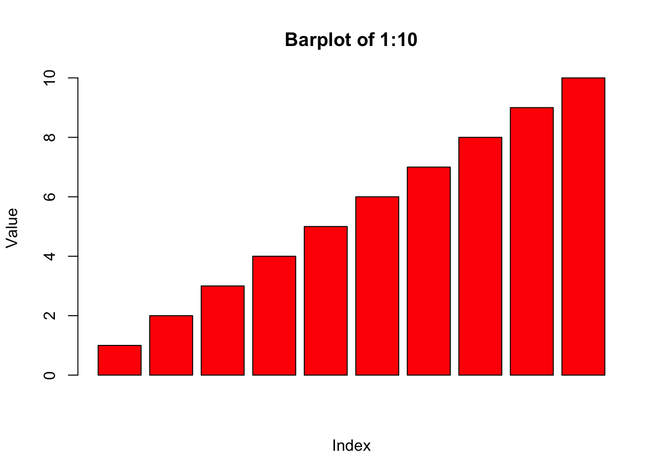
# Create an empirical cumulative distribution function plot
plot.ecdf(rnorm(1000), col = "blue", main = "ECDF of 1000 random normal numbers", xlab = "Value", ylab = "Cumulative Probability")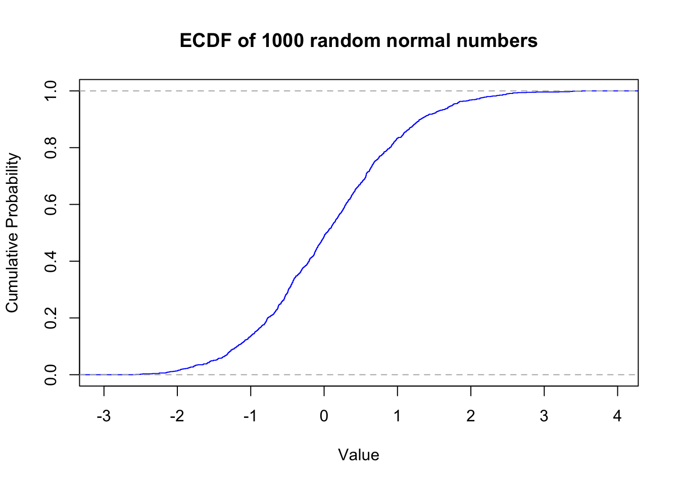
# Get help on the qqplot function
?qqplot
# Create a Q-Q plot comparing x and x^2
x = rnorm(1000)
qqplot(x, x^2)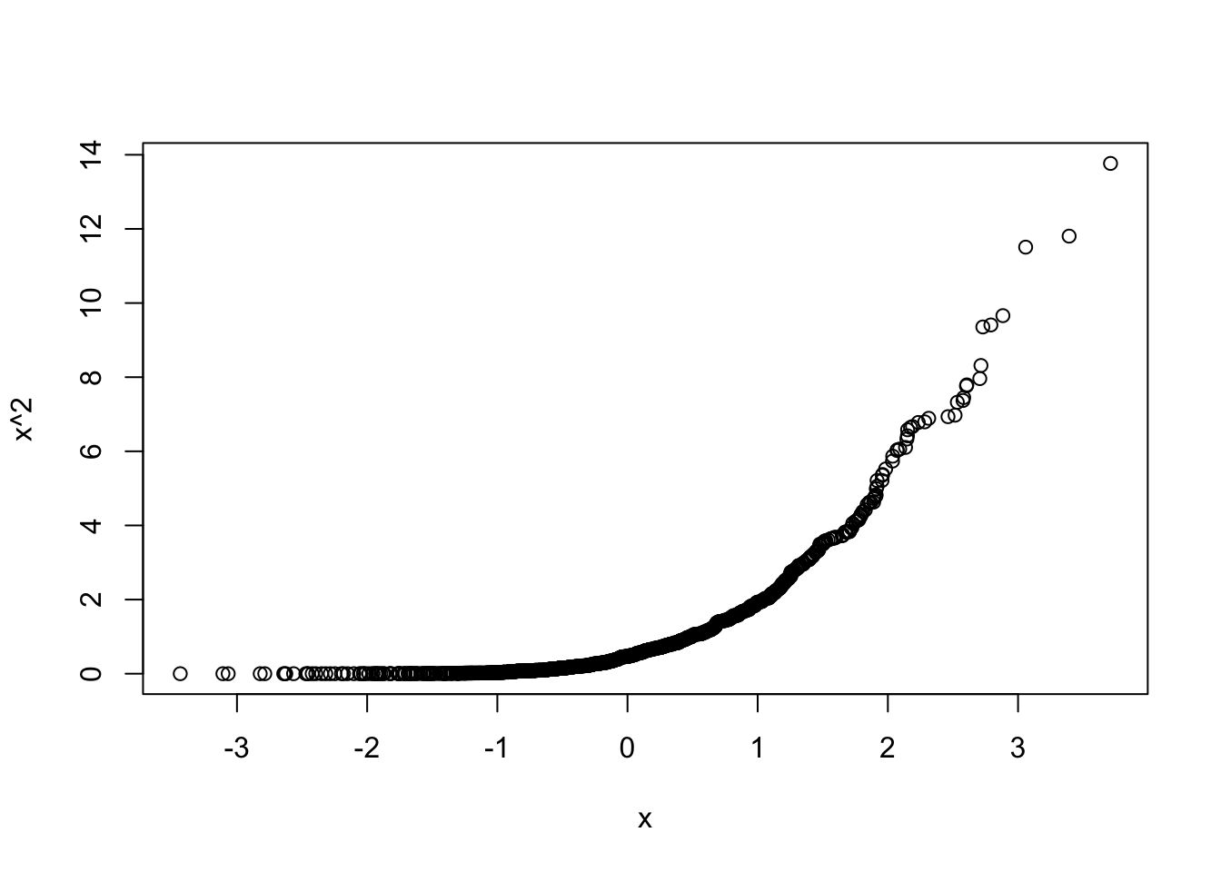
# Create a Q-Q normal plot
qqnorm(x)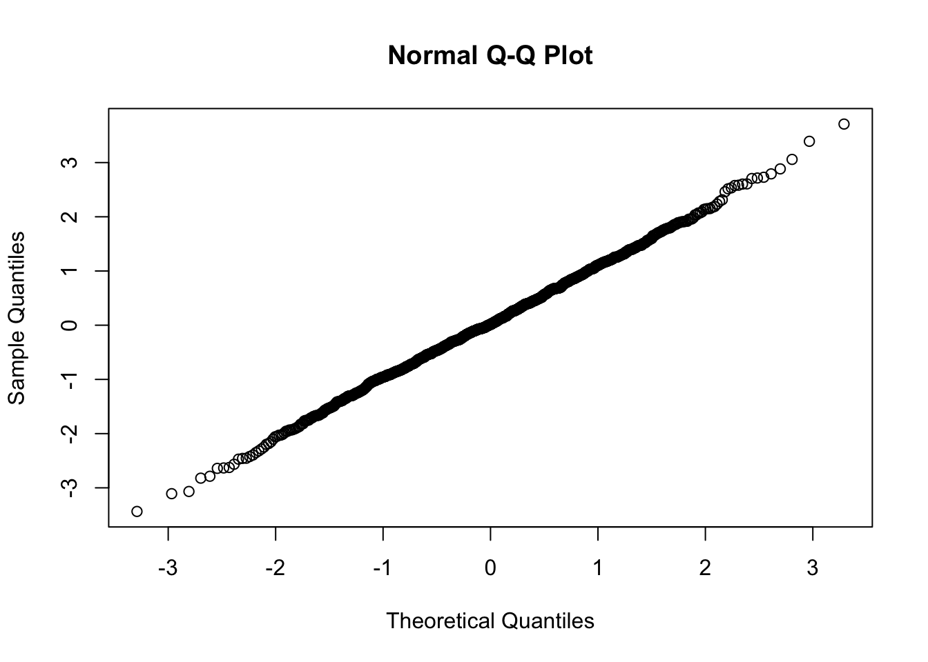
# Get help on the qqline function
?qqline
# Add a Q-Q line to the Q-Q normal plot
# qqline(x, distribution = qnorm)# Create a boxplot of 1000 random normal numbers
boxplot(rnorm(1000), col = "red", main = "Boxplot of 1000 random normal numbers", xlab = "Value", ylab = "Frequency")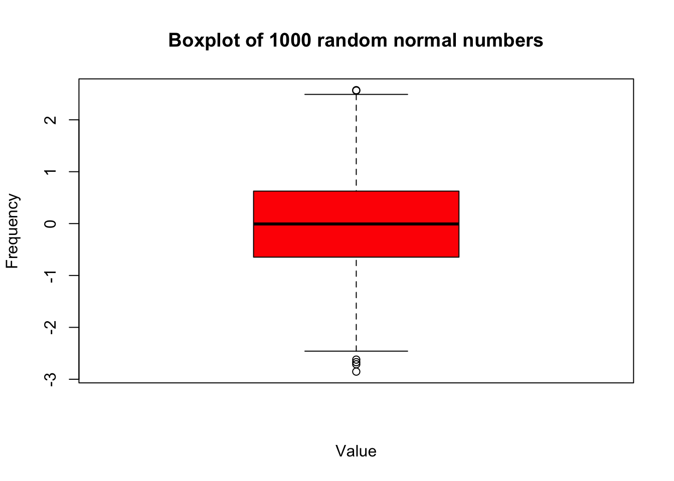
# Create a sample data vector
data <- c(3.1, 4.2, 4.3, 5.4, 5.5, 5.6, 6.7, 7.8, 8.9, 9.0)
# Create a stem-and-leaf plot of the sample data
stem(data)
  The decimal point is at the |

  2 | 1
  4 | 23456
  6 | 78
  8 | 90