Week 8
Normalizing Flows (NFs)
Core Concepts
Definition
- Normalizing Flows (NFs) are generative models that represent a complex data distribution \(p(x)\) by transforming a simple base distribution \(p_Z(z)\) (e.g., Gaussian) through an invertible and differentiable function \(f: \mathcal{Z} \to \mathcal{X}\), where \(x = f(z)\).
Tractable Likelihood
- NFs allow exact likelihood computation using the change of variables formula. Given \(z = f^{-1}(x)\): \[ p_X(x) = p_Z(z) \left| \det \left( \frac{\partial z}{\partial x} \right) \right| = p_Z(f^{-1}(x)) \left| \det J_{f^{-1}}(x) \right| \]
- Alternatively, by the inverse function theorem (\(J_f(z) = (J_{f^{-1}}(x))^{-1}\)): \[ p_X(x) = p_Z(z) \left| \det J_f(z) \right|^{-1} \]
Requirements for Transformation \(f\)
- Invertible: \(f^{-1}\) must exist.
- Differentiable: Both \(f\) and \(f^{-1}\) must be differentiable (i.e., \(f\) is a diffeomorphism).
- Efficient Jacobian Determinant: The determinant of the Jacobian matrix (\(\det J_f\) or \(\det J_{f^{-1}}\)) must be computationally efficient (ideally \(O(D)\) or \(O(D^2)\) for \(D\) dimensions, not \(O(D^3)\) as in the general case). This is often achieved by using triangular or structured Jacobians.
- Dimensionality Preservation: The input and output dimensions must match, i.e., \(\dim(x) = \dim(z)\).
Composition
- Complex transformations are constructed by composing multiple simpler invertible layers: \(f = f_L \circ \dots \circ f_1\).
- The overall log-determinant is the sum of the log-determinants of each layer: \[ \log p_X(x) = \log p_Z(z) + \sum_{i=1}^L \log \left| \det J_{f_i^{-1}}(x_i) \right| \] where \(x_i\) is the input to layer \(f_i^{-1}\).
Inference vs. Sampling
- Likelihood Evaluation (Inference): Compute \(z = f^{-1}(x)\) and evaluate \(p_X(x)\) using the above formula.
- Sampling: Sample \(z \sim p_Z(z)\) and compute \(x = f(z)\).
Key Building Block: Coupling Layers
Concept
- Partition input dimensions \(x\) into two parts, \(x = (x_a, x_b)\). Transform one part (\(x_a\)) based on the other (\(x_b\)), while leaving \(x_b\) unchanged: \[ y_a = h(x_a; \theta(x_b)) \] \[ y_b = x_b \]
- \(h\) must be invertible with respect to \(x_a\).
- \(\theta(x_b)\) can be arbitrarily complex and does not have to be invertible.
Example: Affine Coupling Layer
- \(h(x_a; s, t) = x_a \odot s + t\), where \((s, t) = \theta(x_b)\).
Forward Pass
- \(y_a = h(x_a, \theta(x_b))\)
- \(y_b = x_b\)
Backward Pass
- \(x_a = h^{-1}(y_a, \theta(y_b))\)
- \(x_b = y_b\)
Jacobian Matrix
- The Jacobian is block lower triangular: \[ J = \frac{\partial y}{\partial x} = \begin{pmatrix} \frac{\partial y_a}{\partial x_a} & \frac{\partial y_a}{\partial x_b} \\ 0 & I \end{pmatrix} \]
Determinant
- The determinant is efficient to compute: \[ \det(J) = \det \left( \frac{\partial y_a}{\partial x_a} \right) = \det \left( \frac{\partial h(x_a; \theta(x_b))}{\partial x_a} \right) \]
- For affine coupling layers, \(\frac{\partial y_a}{\partial x_a} = \mathrm{diag}(s)\), so \(\det(J) = \prod_i s_i\).
Conditioning
- To make the flow conditional on external information \(c\), modify the parameter network: \((s, t) = \theta(x_b, c)\). The Jacobian structure remains unchanged.
Transformation Composition
- The overall transformation is a composition of all the transformations, and the determinants multiply (log-determinants sum).
- Since one part of the input is untransformed in each layer, the next layer should transform this part, or at each step, a different mask of features should be used.
Training
- Maximize the exact log-likelihood of i.i.d. samples, so the density is explicitly defined.
Inference
- To sample, draw \(z\) from the base distribution and pass it through the transformations.
- To compute the sample probability, use invertibility to transform \(x\) back to \(z\) and measure its probability.
Continuous Normalizing Flows
- Allow modeling of arbitrarily complex distributions by parameterizing the transformation as a continuous-time ODE.
Architectural Patterns (e.g., RealNVP, GLOW)
General Patterns
- The main differences in architectures are in the choice of \(h\) and how variables are split.
NICE Model
- An early flow-based model using an additive coupling layer and splitting variables as \(x_{1:d}\) and \(x_{d+1:D}\), where \(D\) is the input dimension.
Multi-Scale Architecture
- Employs sequences of blocks operating at different spatial resolutions.
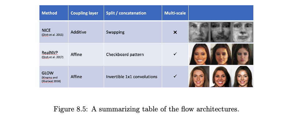
RealNVP
- Utilizes a combination of spatial checkerboard pattern, channel-wise masking, and affine mapping.
- The split operation partitions the input data using a spatial checkerboard pattern, followed by a squeeze operation and channel-wise masking.
- The squeeze operation reduces the spatial dimensions while increasing the number of channels. For an input tensor of size \(W \times H \times C\), the squeeze operation transforms it to \(W/2 \times H/2 \times 4C\) by dividing the input into \(2 \times 2\) subsquares and assigning elements to different channels in a clockwise rotation.
- The coupling layer uses an affine mapping: \[ y_A = x_A \odot \exp(s(x_B)) + t(x_B) \] \[ y_B = x_B \] where \(s\) and \(t\) can be arbitrarily complex (e.g., neural networks), \(\odot\) denotes element-wise product, and \(y_A\), \(y_B\) are the resulting partitions.
- The Jacobian is triangular, so its log-determinant is efficiently computed as \(\sum s(x_B)\).
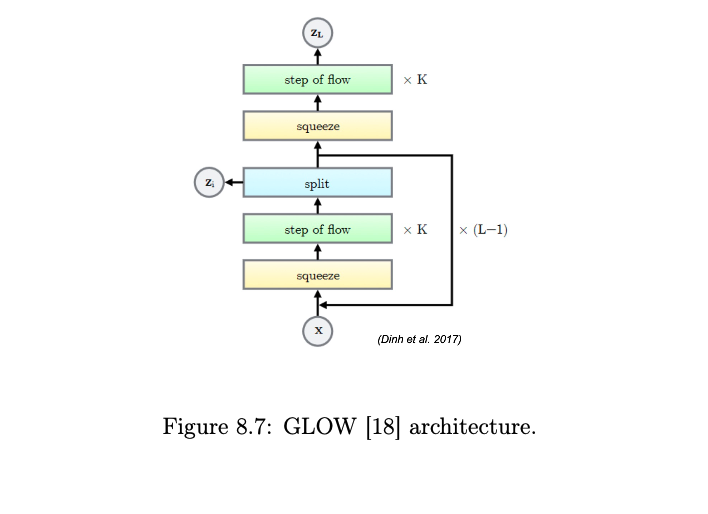
GLOW
Introduced invertible \(1 \times 1\) convolutions and affine coupling layers.
Each flow step consists of:
- Activation Normalization (ActNorm)
- Normalizes each input channel by learning a per-channel scale \(s\) and bias \(b\).
- Forward: \(y_{i,j} = s \odot x_{i,j} + b\)
- Reverse: \(x_{i,j} = (y_{i,j} - b)/s\)
- Log-determinant: \(H \cdot W \cdot \sum \log(|s|)\)
- Invertible \(1 \times 1\) Convolution
- Generalizes permutation in the channel dimension.
- The convolution weight matrix \(W \in \mathbb{R}^{C \times C}\) is initialized as a random rotation matrix with \(\det(W) = 1\).
- To compute the determinant efficiently, \(W\) is parameterized using LU decomposition: \[ W = P \cdot L \cdot (U + \mathrm{diag}(s)) \] where \(P\) is a fixed permutation matrix, \(L\) is lower triangular with ones on the diagonal, \(U\) is upper triangular, and \(s\) is a vector.
- Log-determinant: \(\sum \log |s|\)
- (Conditional) Coupling Layer
- As in RealNVP, but with channel-wise splitting.
- \(x_A, x_B = \mathrm{split}(x)\)
- \((\log s, t) = \mathrm{NN}(x_B)\)
- \(s = \exp(\log s)\)
- \(y_A = s \odot x_A + t\)
- \(y_B = x_B\)
- \(y = \mathrm{concat}(y_A, y_B)\)
- Activation Normalization (ActNorm)
Split Operation
- After a block, a fraction of dimensions (channels) can be split off and passed directly to the latent space \(z\), reducing computational cost in subsequent layers.
Notable NF Models
GLOW
- Introduced invertible \(1 \times 1\) convolutions, achieving high-quality image generation for NFs at the time.
SRFlow
- Uses a conditional NF for super-resolution, modeling \(p(x_{HR} | x_{LR})\).
StyleFlow
- Enables controlled, disentangled editing of images by applying a conditional NF to the latent space (\(\mathcal{W}\) or \(\mathcal{W}+\)) of a pre-trained StyleGAN generator.
- Learns \(w' = f(w; a_{target})\) where \(w\) is the original StyleGAN latent, \(a_{target}\) are desired attributes, and \(w'\) is the edited latent.
- Training uses triplets \(\{w, G(w), A(G(w))\}\), where \(G\) is the StyleGAN generator and \(A\) is an attribute predictor.
- The “forward” pass \(w \to w'\) performs the edit. The “reverse” pass \(w = f^{-1}(w'; a_{target})\) is also possible.
Conditional and Multimodal Flows
Conditional NFs
- Model \(p(x|c)\) by making transformations dependent on conditioning variable \(c\). Used in SRFlow, StyleFlow, etc.
C-Flows (Conditional Flows for Cross-Domain Generation)
- Link multiple data modalities (e.g., images \(x_1\), point clouds \(x_2\)) through a shared latent space \(z\).
- Learn flows \(f_1: \mathcal{X}_1 \to \mathcal{Z}\) and \(f_2: \mathcal{X}_2 \to \mathcal{Z}\).
- Allows generating data in one modality conditioned on another, e.g., generate \(x_2\) from \(x_1\) by computing \(z = f_1^{-1}(x_1)\) and then sampling \(x_2 = f_2(z)\).
- Training can be joint or conditional.
Limitations
Dimensionality Preservation
- Input and output dimensions must match, which can be computationally demanding for high-dimensional data, although techniques like splitting and multi-scale architectures mitigate this.
Sample Quality
- While offering tractable likelihoods, NFs sometimes lag behind Generative Adversarial Networks (GANs) and Diffusion Models in terms of photorealism for complex image generation tasks.
Topology
- Basic NFs cannot change the topology of the space; they are diffeomorphisms. [May not be a practical limitation for many tasks].
Applications in Computer Vision
Super-Resolution
- Learns a distribution of high-resolution variants.
Disentanglement
- Enables disentangled representation learning.
Multimodal Modeling
- Models joint or conditional distributions over multiple modalities.
3D Shape Modeling
- Models complex 3D shapes.
3D Pose Estimation
- Models distributions over 3D poses.
Regularization
- Provides explicit log-likelihoods for regularization in other models.