Week 6
Autoregressive Models
Autoregressive (AR) models factorize a high-dimensional joint distribution into an ordered product of conditionals, enabling exact likelihood computation and principled density estimation.
General Principles
- Factorization
\[p(\mathbf{x}) = \prod_{i=1}^{D} p\bigl(x_i \mid x_{<i}\bigr),\quad x_{<i}=(x_1,\dots,x_{i-1}).\] - Naive Parameterization
- A full tabular representation of each conditional \(p(x_i \mid x_{<i})\) requires \(O(K^D)\) parameters for discrete variables with alphabet size \(K\).
- Alternatively, one could learn \(D\) independent classifiers—one per position—each with its own parameters, giving \(O(D\cdot P)\) parameters for classifier size \(P\).
- Tractable Likelihood
- Exact computation of \(p(\mathbf{x})\) permits maximum likelihood training and direct model comparison.
- Data Modalities
- Sequences (e.g. text): natural ordering
\[p(\text{token}_t \mid \text{tokens}_{<t}).\] - Images: impose scan order (raster, zigzag, diagonal); choice of ordering affects receptive field and modeling capacity.
- Sequences (e.g. text): natural ordering
- Pros & Cons
- Exact density estimation → anomaly detection, likelihood-based evaluation
- Sequential generation in \(O(D)\) steps; slow for high-dimensional \(D\)
- Ordering choice for images is non-trivial
- Comparison to Independence
- Independent model: \(p(\mathbf{x})=\prod_i p(x_i)\) ignores structure but is fast.
Early AR Models for Binary Data
Fully Visible Sigmoid Belief Net (FVSBN)
- Models \(\mathbf{x}\in\{0,1\}^D\) with fixed ordering.
- Conditional logistic regression: \[ p(x_i=1 \mid x_{<i}) = \sigma\!\Bigl(\alpha_i + \sum_{j<i}W_{ij}\,x_j\Bigr). \]
- Parameters: biases \(\{\alpha_i\}_{i=1}^D\) and weights \(W\in\mathbb{R}^{D\times D}\) (upper-triangular).
- Complexity: \(O(D^2)\) parameters, simple but parameter-inefficient.
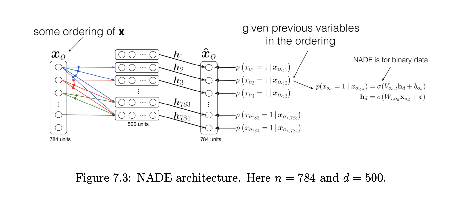
Neural Autoregressive Density Estimator (NADE)
- Shares hidden-layer parameters across all conditionals to reduce complexity from \(O(D^2)\) to \(O(Dd)\), where \(d\) is hidden size.
- Model
- Hidden activations \[ a_1 = c,\quad a_{i+1} = a_i + W_{:,\,i}\,x_i,\quad h_i = \sigma(a_i), \] where \(W\in\mathbb{R}^{d\times D}\) and \(c\in\mathbb{R}^d\) are shared.
- Conditional probability \[ p(x_i=1 \mid x_{<i}) = \hat{x}_i = \sigma\bigl(b_i + V_{i,:}\,h_i\bigr), \] with \(V\in\mathbb{R}^{D\times d}\) and \(b\in\mathbb{R}^D\).
- Properties
- Parameter count: \(O(Dd)\) vs. \(O(D^2)\) in FVSBN
- Computation: joint log-likelihood \(\sum_i\log p(x_i\mid x_{<i})\) in \(O(Dd)\) via one forward pass
- Training
- Maximize average log-likelihood using teacher forcing (use ground-truth \(x_{<i}\)).
- Extensions: RNADE (real-valued inputs), DeepNADE (deep MLP), ConvNADE.
- Inference
- Sequential sampling \(x_1,\dots,x_D\), with optional random ordering for binary pixels.
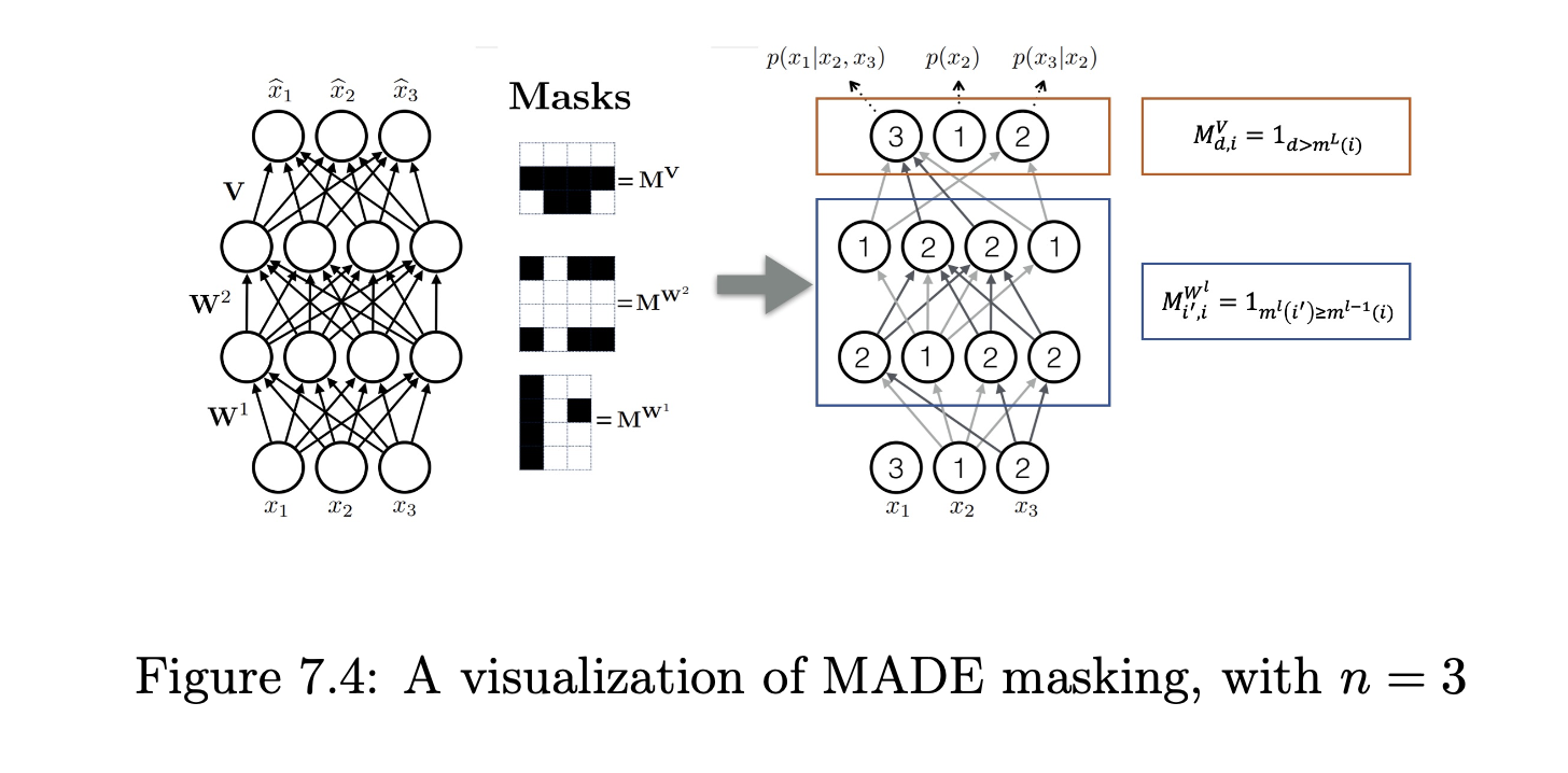
MADE (Masked Autoencoder for Distribution Estimation)
- Adapts a feed-forward autoencoder to AR modeling by masking weights to enforce \(x_i\) depends only on \(x_{<i}\).
- Masking
- Assign each unit an index \(m\in\{1,\dots,D\}\).
- A weight from unit \(u\to v\) is active only if \(m(u)<m(v)\) (hidden layers) and \(m(u)<i\) for output \(x_i\).
- Training & Generation
- Train by minimizing negative log-likelihood.
- Sequential sampling: \(D\) forward passes, one per new \(x_i\).
- Ordering Robustness
- Randomizing masks/orders per epoch improves generalization.
AR Models for Images
PixelRNN
- Uses RNNs (LSTM/GRU) over flattened pixels.
- Dependency: Each pixel \(x_i\) conditioned on RNN hidden state summarizing \(x_{<i}\).
- Ordering: Raster or diagonal scan; variants include Row LSTM, Diagonal BiLSTM.
- Generation: \(O(HW)\) sequential steps for \(H\times W\) image.
PixelCNN
- Uses masked convolutions to model \(p(x_{r,c}\mid x_{\prec(r,c)})\).
- Mask Types
- Type A (first layer): blocks current pixel.
- Type B (subsequent): allows self-connection but no future pixels.
- Training
- Parallel over all pixels via masked convolution stacks.
- Generation
- Sequential sampling \(O(HW)\) steps.
- Blind-Spot Issue
- Deep stacks can leave unconditioned “holes.” Gated PixelCNN or two-pass designs address this.
TCNs (Temporal Convolutional Networks) & WaveNet
- TCN: 1D causal convolutions ensure \(y_t\) depends only on \(x_{\le t}\).
- Dilated Convolutions
- Factor \(d\): gaps between filter taps.
- Stack dilations \(1,2,4,\dots\) for exponential receptive field growth.
- WaveNet
- Masked, dilated convolutions on raw audio.
- Models long-range audio dependencies efficiently.
Variational RNNs (VRNNs) & C-VRNNs
- VRNN
- Embeds a VAE at each timestep \(t\).
- Prior: \(p(z_t\mid h_t)=\mathcal{N}(\mu_{0,t},\mathrm{diag}(\sigma_{0,t}^2))\) where \((\mu_{0,t},\sigma_{0,t})=\phi_{\text{prior}}(h_t)\).
- C-VRNN
- Conditions on external variables (e.g. control signals) alongside latent \(z_t\).
Architecture Trade-offs for \(p(x_i\mid x_{<i})\)
- RNNs
- Compress arbitrary history.
- Recency bias; vanishing distant signals.
- CNNs (Masked/Dilated)
- Parallelizable; scalable receptive field.
- Fixed context; blind spots.
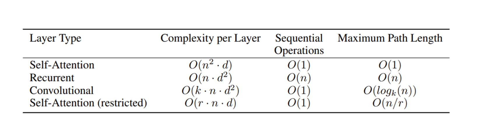
- Transformers
- Masked self-attention to all \(x_{<i}\).
- Highly parallel training.
- Quadratic \(O(L^2)\) attention cost; need positional encoding.
- Large Language Models (LLMs)
- Transformer-based AR on token sequences.
- Pretraining: next-token prediction.
- Fine-Tuning: supervised tasks (SFT).
- Tokenization: subword units (BPE, WordPiece).
AR for High-Resolution Images & Video
- Challenge: Millions of pixels/voxels → \(O(D)\) sequential steps infeasible.
- Approach: Compress data into discrete latent sequences via VQ-VAE.
Vector-Quantized VAE (VQ-VAE)
Objective: Learn a discrete latent representation for high-dimensional data, enabling compact encoding and efficient autoregressive modeling.
Model Components:
- Encoder:
- A convolutional neural network (CNN) mapping input
\(\mathbf{x}\in\mathbb{R}^{H\times W\times C}\) to continuous latents
\(\mathbf{z}_e(\mathbf{x})\in\mathbb{R}^{H'\times W'\times D}\). - Spatial down-sampling factor \(s\): \(H'=H/s,\;W'=W/s\) (e.g. \(s=8\)).
- A convolutional neural network (CNN) mapping input
- Codebook:
- A collection \(\mathcal{E}=\{e_j\in\mathbb{R}^D\mid j=1,\dots,K\}\) of \(K\) trainable embedding vectors.
- Quantization:
- For each spatial cell \((p,q)\), take
\(z_e(\mathbf{x})_{p,q}\in\mathbb{R}^D\) and find nearest codebook index \[ k_{p,q} = \arg\min_{j\in\{1..K\}} \bigl\|z_e(\mathbf{x})_{p,q} - e_j\bigr\|_2^2. \] - Replace \(z_e(\mathbf{x})_{p,q}\) with \(e_{k_{p,q}}\), yielding discrete latents
\(\mathbf{z}_q(\mathbf{x})\in\mathbb{R}^{H'\times W'\times D}\).
- For each spatial cell \((p,q)\), take
- Decoder:
- A CNN mapping \(\mathbf{z}_q(\mathbf{x})\) back to a reconstruction
\(\hat{\mathbf{x}}\in\mathbb{R}^{H\times W\times C}\).
- A CNN mapping \(\mathbf{z}_q(\mathbf{x})\) back to a reconstruction
- Encoder:
Loss Terms:
- Reconstruction Loss: \[ L_{\mathrm{rec}} = \bigl\|\mathbf{x} - \hat{\mathbf{x}}\bigr\|_2^2. \]
- Codebook Loss: (fix encoder, update codebook) \[ L_{\mathrm{cb}} = \sum_{p,q} \bigl\|\mathrm{sg}\bigl[z_e(\mathbf{x})_{p,q}\bigr] - e_{k_{p,q}}\bigr\|_2^2. \]
- Commitment Loss: (fix codebook, update encoder) \[ L_{\mathrm{com}} = \beta \sum_{p,q} \bigl\|z_e(\mathbf{x})_{p,q} - \mathrm{sg}\bigl[e_{k_{p,q}}\bigr]\bigr\|_2^2, \] where \(\beta\) (e.g. \(0.25\)) balances encoder commitment, and \(\mathrm{sg}[\cdot]\) is stop‐gradient.
- Total Loss: \[ L_{\mathrm{VQ\text{-}VAE}} = L_{\mathrm{rec}} + L_{\mathrm{cb}} + L_{\mathrm{com}}. \]
Optimization Details:
- Straight-Through Estimator (STE):
- Quantization is non-differentiable.
- In backprop, pass gradients from \(\mathbf{z}_q\) directly to \(\mathbf{z}_e\) (i.e. treat quantization as identity).
- Codebook Updates via EMA (alternatively):
- Maintain per‐embedding counts \(N_j\) and sums \(m_j\): \[ N_j \gets \gamma\,N_j + (1-\gamma)\sum_{p,q}\mathbf{1}[k_{p,q}=j], \] \[ m_j \gets \gamma\,m_j + (1-\gamma)\sum_{p,q:k_{p,q}=j} z_e(\mathbf{x})_{p,q}, \] then update \[ e_j \gets \frac{m_j}{N_j}, \] with decay \(\gamma\approx0.99\).
- Straight-Through Estimator (STE):
Practical Considerations:
- Hyperparameters:
- Codebook size \(K\) (e.g. 512–1024), embedding dimension \(D\) (e.g. 64–256).
- Compression factor \(s\) reduces sequence length from \(HW\) to \(H'W'\).
- Downstream Use:
- After training, the discrete codes \(\{k_{p,q}\}\) form a sequence of length \(H'W'\).
- An autoregressive model (e.g. Transformer) can be trained on these code sequences:
\[p(k_{p,q}\mid k_{<p,q}).\]
- Intuition:
- Each \(e_j\) becomes a “prototype” latent vector.
- The encoder emits a continuous vector, which is snapped to its nearest prototype, enforcing discreteness and preventing posterior collapse.
- Hyperparameters: