Week 4
Recurrent Neural Networks (RNNs)
Recurrent Neural Networks (RNNs) are a class of artificial neural networks designed specifically for processing sequential data. Unlike feedforward neural networks, RNNs possess internal memory (state) that allows them to capture temporal dependencies and patterns over time.
Key Characteristics:
- Sequential Data Processing: Suited for tasks where the order of input elements matters, such as time series, natural language, speech, and video.
- Variable-Length Sequences: Can naturally handle input and output sequences of varying lengths.
- Internal State (Memory): Maintain a hidden state \(h^t\) that is updated at each time step, summarizing information from past inputs in the sequence. This state is recurrently fed back into the network.
- Weight Sharing: The same set of weights is used across all time steps for processing different elements of the sequence. This allows the model to generalize to sequences of different lengths and learn patterns that are consistent across time.
Common RNN Architectures based on Input/Output Mapping:
- One-to-One: Standard feedforward neural network (not typically considered an RNN in this context, but serves as a baseline).
- Example: Image classification (single input, single output).
- One-to-Many: A single input generates a sequence of outputs.
- Example: Image captioning (input: image; output: sequence of words).
- Example: Music generation from a seed note.
- Many-to-One: A sequence of inputs generates a single output.
- Example: Sentiment analysis (input: sequence of words; output: sentiment label).
- Example: Sequence classification (e.g., classifying a video based on its frames).
- Many-to-Many (Synchronous): A sequence of inputs generates a corresponding sequence of outputs, with alignment between input and output at each step.
- Example: Video frame classification (classifying each frame in a video).
- Example: Part-of-speech tagging (tagging each word in a sentence).
- Many-to-Many (Asynchronous/Delayed): A sequence of inputs generates a sequence of outputs, but the lengths may differ, and alignment is not necessarily one-to-one at each step.
- Example: Machine translation (input: sentence in one language; output: sentence in another language).
- Example: Speech recognition (input: audio sequence; output: sequence of words).
- One-to-One: Standard feedforward neural network (not typically considered an RNN in this context, but serves as a baseline).
RNNs as Dynamical Systems
RNNs can be viewed as discrete-time dynamical systems.
- Dynamical System Definition: A mathematical model describing the temporal evolution of a system’s state. The state at a given time is a function of its previous state and any external inputs.
- Continuous-time dynamical systems are often described by differential equations (e.g., \(\frac{dh(t)}{dt} = f(h(t), x(t))\)).
- RNNs are discrete-time dynamical systems, where the state \(h^t\) evolves at discrete time steps \(t\). The evolution is defined by a recurrence relation: \[ h^t = f(h^{t-1}, x^t; \theta) \] where \(h^t\) is the hidden state at time \(t\), \(h^{t-1}\) is the hidden state at the previous time step, \(x^t\) is the input at time \(t\), and \(\theta\) represents the model parameters (weights and biases).
- Relation to Hidden Markov Models (HMMs): While both RNNs and HMMs model sequences and have hidden states, they are different concepts. HMMs are probabilistic graphical models with discrete states and explicit transition/emission probabilities. RNNs are connectionist models with continuous hidden states and learn transitions implicitly through neural network functions. HMMs are a specific type of dynamical system, but not all discrete dynamical systems are HMMs.
Vanilla RNN
The “vanilla” RNN is the simplest form of a recurrent network.
State Update Equation: The hidden state \(h^t\) is computed as a non-linear function of the previous hidden state \(h^{t-1}\) and the current input \(x^t\):
\[ h^t = \tanh(W_{hh} h^{t-1} + W_{xh} x^t + b_h) \]
where:
- \(x^t\) is the input vector at time step \(t\).
- \(h^{t-1}\) is the hidden state vector from the previous time step \(t-1\).
- \(W_{xh}\) is the weight matrix connecting the input to the hidden layer.
- \(W_{hh}\) is the weight matrix connecting the previous hidden state to the current hidden state (the recurrent weights).
- \(b_h\) is the bias vector for the hidden layer.
- \(\tanh\) is the hyperbolic tangent activation function.
Output Equation: The output \(\hat{y}^t\) at time step \(t\) is typically computed from the current hidden state:
\[ \hat{y}^t = W_{hy} h^t + b_y \]
where:
- \(W_{hy}\) is the weight matrix connecting the hidden layer to the output layer.
- \(b_y\) is the bias vector for the output layer.
Weight Sharing: The weight matrices (\(W_{xh}, W_{hh}, W_{hy}\)) and biases (\(b_h, b_y\)) are shared across all time steps.
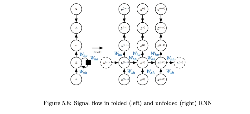
- Training: Backpropagation Through Time (BPTT)
- BPTT unrolls the RNN through time for a sequence of length \(S\) and applies backpropagation.
- The total loss \(L\) is the sum of losses \(L^t\) at each time step (e.g., \(L^t = \|\hat{y}^t - y^t\|^2\)).
- The gradient of the total loss \(L\) with respect to any weight matrix \(W\) is: \[ \frac{\partial L}{\partial W} = \sum_{t=1}^{S} \frac{\partial L^t}{\partial W} \]
- The gradient of the loss at a specific time step \(t\), \(L^t\), with respect to \(W\) is found by summing influences through all intermediate hidden states \(h^k\): \[ \frac{\partial L^t}{\partial W} = \sum_{k=1}^{t} \frac{\partial L^t}{\partial \hat{y}^t} \frac{\partial \hat{y}^t}{\partial h^t} \frac{\partial h^t}{\partial h^k} \frac{\partial^+ h^k}{\partial W} \] where \(\frac{\partial^+ h^k}{\partial W}\) is the “immediate” partial derivative.
- Vanishing/Exploding Gradients: The term \(\frac{\partial h^t}{\partial h^k}\) is critical: \[
\frac{\partial h^t}{\partial h^k} = \prod_{i=k+1}^{t} \frac{\partial h^i}{\partial h^{i-1}}
\] Given the state update \(h^i = \tanh(W_{hh} h^{i-1} + W_{xh} x^i + b_h)\), the Jacobian is: \[
\frac{\partial h^i}{\partial h^{i-1}} = W_{hh} \operatorname{diag}(1 - (h^{i-1})^2)
\] where \(\operatorname{diag}(1 - (h^{i-1})^2)\) is a diagonal matrix with entries \(1 - (h^{i-1}_j)^2\). Thus, the product becomes: \[
\frac{\partial h^t}{\partial h^k} = \prod_{i=k+1}^{t} \left( W_{hh} \operatorname{diag}(1 - (h^{i-1})^2) \right)
\] This product involves repeated multiplication of \(W_{hh}\) (and diagonal matrices).
- If the magnitudes of eigenvalues/singular values of \(W_{hh}\) are consistently greater than 1, the norm of this product can grow exponentially with \(t-k\), leading to exploding gradients.
- If they are consistently less than 1, the norm can shrink exponentially, leading to vanishing gradients.
Long Short-Term Memory (LSTM)
LSTMs were introduced by Sepp Hochreiter and Jürgen Schmidhuber in 1997 to address the vanishing gradient problem in vanilla RNNs. They achieve this through a more complex internal cell structure involving gating mechanisms.
- Core Idea: LSTMs use gates (input, forget, output) to control the flow of information into and out of a cell state \(c_t\). The cell state acts as a memory conveyor belt, allowing information to propagate over long durations with minimal decay.
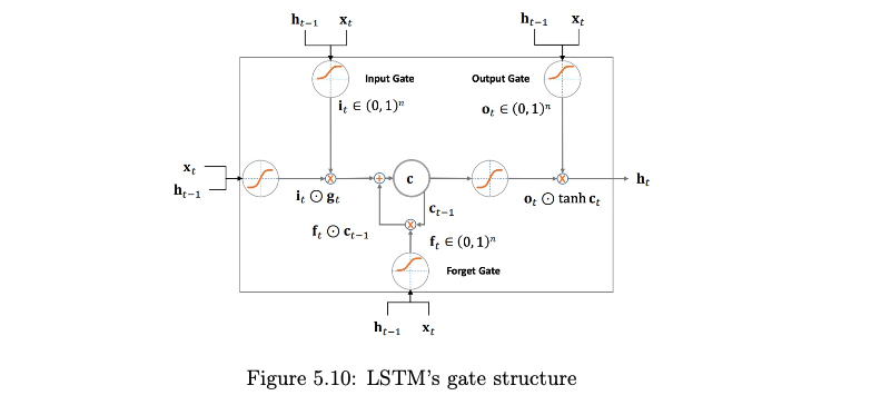
Matrix Representation for Gates and Cell Update: Let \(x_t\) be the current input and \(h_{t-1}\) be the previous hidden state. The core computations for the gates (forget \(f_t\), input \(i_t\), output \(o_t\)) and the candidate cell state \(\tilde{c}_t\) can be combined:
\[ \begin{pmatrix} i_t \\ f_t \\ o_t \\ \tilde{c}_t \end{pmatrix} = \begin{pmatrix} \sigma \\ \sigma \\ \sigma \\ \tanh \end{pmatrix} \left( W \begin{bmatrix} x_t \\ h_{t-1} \end{bmatrix} + b \right) \]
where \(W\) is a block weight matrix and \(b\) is a block bias vector. The cell state \(c_t\) and hidden state \(h_t\) are then updated:
\[ c_t = f_t \odot c_{t-1} + i_t \odot \tilde{c}_t \]
\[ h_t = o_t \odot \tanh(c_t) \]
where \(\sigma\) is the sigmoid function, \(\tanh\) is the hyperbolic tangent function, and \(\odot\) denotes element-wise multiplication.
Stacked LSTMs (Multiple Layers): LSTMs can be stacked to create deeper recurrent networks. The hidden state \(h_t^{[l]}\) of layer \(l\) at time \(t\) becomes the input \(x_t^{[l+1]}\) for layer \(l+1\) at the same time step \(t\).
Gated Recurrent Unit (GRU)
The Gated Recurrent Unit (GRU), introduced by Cho et al. in 2014, is a variation of the LSTM with a simpler architecture and fewer parameters. It often performs comparably to LSTMs on many tasks.
- Key Differences from LSTM:
- It combines the forget and input gates of an LSTM into a single update gate.
- It merges the cell state and hidden state, resulting in only one state vector being passed between time steps.
- It uses a reset gate to control how much of the previous state information is incorporated into the candidate state.
- GRUs are generally computationally slightly more efficient than LSTMs due to having fewer gates and parameters. The choice between LSTM and GRU often depends on the specific dataset and task, with empirical evaluation being the best guide.
Gradient Clipping
Gradient clipping is a common technique used during the training of RNNs (and other deep networks) to mitigate the exploding gradient problem.
- Mechanism:
- If the L2 norm of the gradient vector \(g = \frac{\partial L}{\partial W}\) (where \(W\) represents all parameters, or parameters of a specific layer) exceeds a predefined threshold \(\tau\), the gradient is scaled down to have a norm equal to \(\tau\).
- If \(\|g\|_2 > \tau\), then \(g \leftarrow \frac{\tau}{\|g\|_2} g\).
- If \(\|g\|_2 \le \tau\), then \(g\) remains unchanged.
- Purpose: It prevents excessively large gradient updates that can destabilize the training process, without changing the direction of the gradient. It does not directly solve the vanishing gradient problem.