Week 3
Convolutional Neural Networks (CNNs)
Convolutional Neural Networks (CNNs) are a class of deep neural networks particularly well-suited for processing grid-like data, such as images.
- Wide Range of Applications:
- Image classification, object localization, instance segmentation, semantic segmentation, 3D pose estimation, eye gaze estimation, dynamic gesture recognition, and more.
- Biological Inspiration:
- CNNs are inspired by the organization of the animal visual cortex.
- Hubel and Wiesel (1950s-1960s) discovered a hierarchy in the visual cortex:
- Simple cells: Respond to specific features (e.g., oriented edges) at particular locations; susceptible to noise.
- Complex cells: Aggregate responses from simple cells, providing spatial invariance and robustness.
- Neocognitron (Fukushima, 1980):
- Early hierarchical neural network model for visual pattern recognition.
- S-cells: Simple cells, analogous to convolutional filters.
- C-cells: Complex cells, analogous to pooling layers.
The Convolution Operation in CNNs
- Properties:
- Linear transformation.
- Shift equivariance: Shifting the input shifts the output in the same way.
- Mathematical Definition (Convolution):
- Given input image \(I\) and kernel \(K\), the output \(I'\) is: \[ I'(i, j) = \sum_{m} \sum_{n} K(m, n) \, I(i - m, j - n) \]
- Cross-Correlation (as used in most deep learning libraries): \[
I'(i, j) = \sum_{m} \sum_{n} K(m, n) \, I(i + m, j + n)
\]
- True convolution is cross-correlation with a 180-degree rotated kernel: \(I * K = I \star K_{\text{flipped}}\), where \(K_{\text{flipped}}(m, n) = K(-m, -n)\).
- Commutativity: Convolution is commutative (\(I * K = K * I\)), cross-correlation is not.
CNN Architecture Overview
A typical CNN consists of:
- Convolutional layers: Learn spatial features.
- Activation functions: Non-linearities (e.g., ReLU, sigmoid, tanh).
- Pooling layers: Downsample feature maps.
- Fully connected layers: Used at the end for classification/regression.
Mathematical Derivation of a Convolutional Layer
Let \(z^{[l-1]}_{u, v}\) be the output of layer \(l-1\) at position \((u, v)\). Let \(w^{[l]}_{m, n}\) be the filter weights, and \(b^{[l]}\) the bias.
Forward Pass:
\[ z^{[l]}_{i, j} = \sum_{m} \sum_{n} w^{[l]}_{m, n} \, z^{[l-1]}_{i - m, j - n} + b^{[l]} \]
Backward Pass:
Let \(L\) be the loss, and \(\delta^{[l]}_{i, j} = \frac{\partial L}{\partial z^{[l]}_{i, j}}\).
Gradient w.r.t. previous layer activations:
\[ \delta^{[l-1]}_{i, j} = \sum_{m} \sum_{n} \delta^{[l]}_{i + m, j + n} \, w^{[l]}_{m, n} \]
- This is equivalent to convolving \(\delta^{[l]}\) with the kernel \(w^{[l]}\) rotated by 180 degrees: \[ \delta^{[l-1]} = \delta^{[l]} * \text{rot180}(w^{[l]}) \]
Gradient w.r.t. weights:
\[ \frac{\partial L}{\partial w^{[l]}_{m, n}} = \sum_{i} \sum_{j} \delta^{[l]}_{i, j} \, z^{[l-1]}_{i - m, j - n} \]
- This is the cross-correlation of \(z^{[l-1]}\) with \(\delta^{[l]}\).
Gradient w.r.t. bias: \[ \frac{\partial L}{\partial b^{[l]}} = \sum_{i} \sum_{j} \delta^{[l]}_{i, j} \]
Pooling Layers
- Purpose: Downsample feature maps, reduce computation, and provide translation invariance.
- Max pooling: Takes the maximum value in a local region.
- No parameters.
- During backpropagation, the gradient is passed only to the input that had the maximum value.
- Average pooling: Takes the average value in a local region.
- Modern trend: Strided convolutions often replace pooling.
Convolution and Cross-Correlation Identities
- \(A * \text{rot180}(B) = A \star B\)
- \(A \star B = \text{rot180}(B) * A\)
Fully Convolutional Networks (FCNs)
- Semantic segmentation: Classify each pixel.
- Input and output dimensions: Typically the same.
- Architecture: Downsample (encoder), then upsample (decoder).
- Upsampling methods:
- Fixed: Nearest neighbor, “bed of nails”, max unpooling.
- Learnable: Transposed convolution.
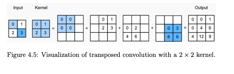
Transposed Convolution
- Also called: Fractionally strided convolution, “deconvolution” (not a true inverse).
- Mechanism:
- Upsample by inserting zeros between input elements.
- Apply a standard convolution to the upsampled input.
- Output size for input height \(H_{in}\), kernel size \(k\), stride \(s\), and padding \(p\): \[ H_{out} = s (H_{in} - 1) + k - 2p \]
- Visualization: Each input value is multiplied by the kernel and “spread” over the output, overlapping values are summed.
U-Net Architecture
- Symmetric encoder-decoder: Contracting path (encoder) for context, expanding path (decoder) for localization.
- Skip connections: Concatenate encoder features with decoder features at corresponding resolutions for better localization.
- Applications: Semantic segmentation, image generation from segmentation maps, 3D human pose/shape estimation, and more.