Implicit Surfaces, Neural Radiance Fields (NeRFs), and 3D Gaussian Splatting
- This lecture extends 2D model generation concepts to 3D, focusing on representations, rendering, and learning methods for 3D scenes.
3D Representations
- Voxels
- Discretize 3D space into a regular grid of volumetric pixels (voxels).
- Memory complexity is cubic: \(O(N^3)\) for an \(N \times N \times N\) grid.
- Resolution is limited by grid size.
- Point Primitives / Volumetric Primitives
- Represent geometry as a collection of points (point cloud) or simple volumetric shapes (e.g., spheres).
- Do not explicitly encode connectivity or topology.
- Easily acquired with depth sensors (e.g., LiDAR).
- Meshes
- Composed of vertices (points), edges (connections), and faces (typically triangles).
- Limited by the number of vertices; low resolution can cause self-intersections.
- Some methods require class-specific templates, but general mesh learning is also common.
- Remain popular due to compatibility with standard rendering pipelines.
Implicit Surfaces
- Explicit vs. Implicit Shape Representation
- Explicit (mesh-like): Defined by discrete vertices and faces; representation is discontinuous.
- Implicit: Defined by a function \(f(x, y) = 0\) (e.g., a circle: \(x^2 + y^2 - r^2 = 0\)); representation is continuous.
- To compute \(\frac{dy}{dx}\) for \(F(x, y) = 0\) (e.g., \(x^2 + y^2 - 1 = 0\)): \[
\begin{aligned}
\frac{d}{dx}[x^2 + y^2] &= \frac{d}{dx}[1] \\
2x + 2y \frac{dy}{dx} &= 0 \\
\frac{dy}{dx} &= -\frac{x}{y}
\end{aligned}
\]
- More generally, for \(F(x, y) = 0\): \[
\frac{dy}{dx} = -\frac{\partial F / \partial x}{\partial F / \partial y}
\] (assuming \(\partial F / \partial y \neq 0\)).
- Level Sets
- Represent the surface as the zero level set of a continuous function \(f: \mathbb{R}^3 \to \mathbb{R}\): \[
S = \{ \mathbf{x} \in \mathbb{R}^3 \mid f(\mathbf{x}) = 0 \}
\]
- \(f\) can be approximated by a neural network \(f_\theta(\mathbf{x})\).
- Signed Distance Functions (SDFs)
- \(f(\mathbf{x})\) gives the signed distance from \(\mathbf{x}\) to the surface; sign indicates inside/outside.
- Storing SDFs on a grid leads to \(O(N^3)\) memory and limited resolution.
- Neural Implicit Representations (e.g., Occupancy Networks, DeepSDF)
- Neural network predicts occupancy probability or SDF value for any \(\mathbf{x} \in \mathbb{R}^3\).
- Can be conditioned on class labels or images.
- Advantages:
- Low memory (just network weights).
- Continuous, theoretically infinite resolution.
- Can represent arbitrary topologies.
Neural Fields
- Neural fields generalize neural implicit representations to predict not only geometry but also color, lighting, and other properties.
- Surface Normals from SDFs
- Surface normal at \(\mathbf{x}\): \(\mathbf{n}(\mathbf{x}) = \nabla f(\mathbf{x}) / \| \nabla f(\mathbf{x}) \|\).
- Computed efficiently via auto-differentiation.
- Used for regularization (e.g., Eikonal term).
Training Neural Implicit Surfaces
- Supervision Levels (from easiest to hardest for geometry learning):
- Watertight Meshes
- Sample points and query occupancy or SDF.
- Train with cross-entropy (occupancy) or regression (SDF).
- Point Clouds
- Supervise so that \(f_\theta(\mathbf{x}) \approx 0\) for observed points.
- Images
- Requires differentiable rendering to compare rendered and real images.
- Visualizing Implicit Surfaces
- Evaluate \(f_\theta(\mathbf{x})\) on a grid and extract a mesh (e.g., Marching Cubes).
- Overfitting for Representation
- Networks can be trained to overfit a single shape/class, compressing it into the weights.
- For implicit surfaces, this means accurate 3D reconstruction, not novel view synthesis.
- Eikonal Regularization
- Enforces \(\| \nabla f(\mathbf{x}) \| = 1\) for SDFs.
- Encourages smooth, well-behaved level sets.
- Loss: \[
L = \sum_{\mathbf{x}} |f_\theta(\mathbf{x})| + \lambda \sum_{\mathbf{x}} (\| \nabla f_\theta(\mathbf{x}) \| - 1)^2
\]
- Alternatively, an L1 penalty: \[
L = \sum_{\mathbf{x}} |f_\theta(\mathbf{x})| + \lambda \sum_{\mathbf{x}} |\| \nabla f_\theta(\mathbf{x}) \| - 1|
\]
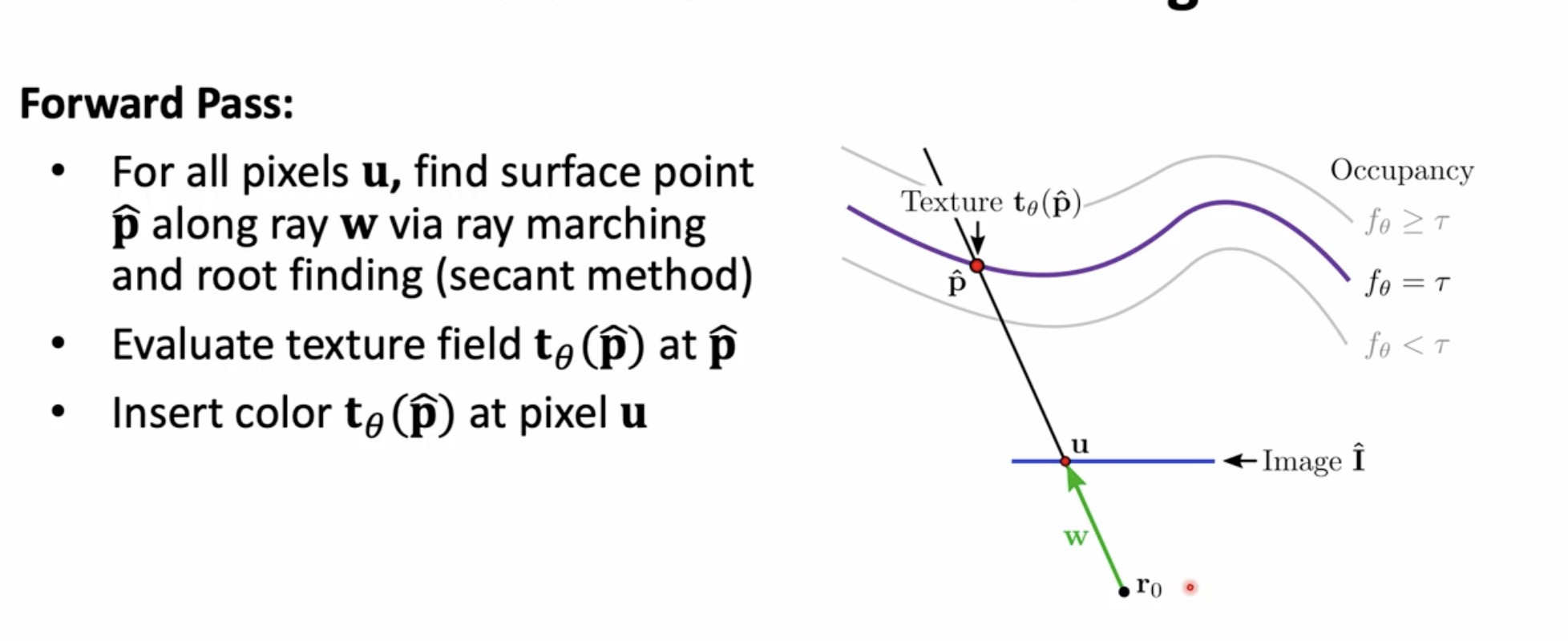
Differentiable Rendering for Neural Fields
- Goal: Learn \(f_\theta\) (geometry) and \(t_\theta\) (texture) from 2D images by rendering and comparing to ground truth.
- Rendering Pipeline:
- For each pixel \(u\), cast a ray \(\mathbf{r}(d) = \mathbf{r}_0 + \mathbf{w}d\).
- Find intersection \(\hat{\mathbf{p}}\) where \(f_\theta(\hat{\mathbf{p}}) = \tau\) (e.g., \(\tau = 0\)).
- Use root-finding (e.g., Secant method) between samples with opposite signs.
- Query \(t_\theta(\hat{\mathbf{p}})\) for color.
- Assign color to pixel \(u\).
- Forward Pass:
- Backward Pass:
- For loss \(L(I, \hat{I}) = \sum_u \| \hat{I}_u - I_u \|_1\).
- Where \(\hat{I}_u = t_\theta(\hat{\mathbf{p}})\) is the rendered color at pixel \(u\), where both \(t_\theta\) and \(\hat{\mathbf{p}}\) depend on \(\theta\). \[
\frac{\partial \hat{I}_u}{\partial \theta} = \frac{\partial t_\theta(\hat{\mathbf{p}})}{\partial \theta} + \nabla_{\hat{\mathbf{p}}} t_\theta(\hat{\mathbf{p}}) \cdot \frac{\partial \hat{\mathbf{p}}}{\partial \theta}
\]
- Implicit differentiation for \(\frac{\partial \hat{\mathbf{p}}}{\partial \theta}\): \[
f_\theta(\hat{\mathbf{p}}) = \tau \implies \frac{\partial f_\theta(\hat{\mathbf{p}})}{\partial \theta} + \nabla_{\hat{\mathbf{p}}} f_\theta(\hat{\mathbf{p}}) \cdot \frac{\partial \hat{\mathbf{p}}}{\partial \theta} = 0
\] \[
\frac{\partial \hat{\mathbf{p}}}{\partial \theta} = -\frac{\frac{\partial f_\theta(\hat{\mathbf{p}})}{\partial \theta}}{\nabla_{\hat{\mathbf{p}}} f_\theta(\hat{\mathbf{p}}) \cdot \mathbf{w}} \mathbf{w}
\]
Neural Radiance Fields (NeRFs)
- Motivation: Model complex scenes with thin structures, transparency, and view-dependent effects.
- Task: Given images with known camera poses, learn a volumetric scene representation for novel view synthesis.
- Network Architecture:
- Input: 3D point \(\mathbf{x}\) and viewing direction \(\mathbf{d}\).
- Output: Color \(\mathbf{c}\) and density \(\sigma\).
- Structure:
- \(\mathbf{x}\) (after positional encoding) passes through several fully connected layers.
- Outputs \(\sigma\) and a feature vector.
- \(\mathbf{d}\) (after positional encoding) is concatenated with the feature vector.
- Final layers output view-dependent color \(\mathbf{c}\).
- Density \(\sigma\) depends only on \(\mathbf{x}\); color \(\mathbf{c}\) depends on both \(\mathbf{x}\) and \(\mathbf{d}\).
- Positional Encoding:
- MLPs are biased toward low-frequency functions.
- Encode each input coordinate \(p\) as: \[
\gamma(p) = (\sin(2^0 \pi p), \cos(2^0 \pi p), \ldots, \sin(2^{L-1} \pi p), \cos(2^{L-1} \pi p))
\]
- Typically \(L=10\) for \(\mathbf{x}\), \(L=4\) for \(\mathbf{d}\).
- Volume Rendering Process:
- For each pixel, cast a ray \(\mathbf{r}(t) = \mathbf{o} + t\mathbf{d}\).
- Sample \(N\) points along the ray.
- For each sample \(i\) at \(t_i\):
- Query MLP: \((\mathbf{c}_i, \sigma_i) = \text{MLP}(\mathbf{r}(t_i), \mathbf{d})\).
- Compute \(\delta_i = t_{i+1} - t_i\).
- Compute opacity: \(\alpha_i = 1 - \exp(-\sigma_i \delta_i)\).
- Compute transmittance: \(T_i = \prod_{j=1}^{i-1} (1 - \alpha_j)\), with \(T_1 = 1\).
- Color Integration: \[
\hat{C}(\mathbf{r}) = \sum_{i=1}^{N} T_i \alpha_i \mathbf{c}_i
\]
- \(N\): Number of samples along the ray.
- \(\mathbf{c}_i, \sigma_i\): Color and density from MLP at sample \(i\).
- \(\delta_i\): Distance between samples.
- \(\alpha_i\): Opacity for interval \(i\).
- \(T_i\): Transmittance up to sample \(i\).
- Hierarchical Volume Sampling (HVS):
- Use a coarse network to sample uniformly, then a fine network to sample more densely where \(T_i \alpha_i\) is high.
- Training & Characteristics:
- Volumetric, models transparency and thin structures.
- Geometry can be noisy compared to explicit surface methods.
- Requires many calibrated images.
- Rendering is slow due to many MLP queries.
- Original NeRF is for static scenes.
- Animating NeRFs / Dynamic Scenes
- Use a canonical space (e.g., T-pose) and learn a deformation field to map to observed poses.
- Find correspondences between observed and canonical space (may require a separate network).
- If multiple correspondences, select or aggregate (e.g., max confidence) [Verification Needed].
- Example: Vid2Avatar.
- Alternative Parametrizations
- Use explicit primitives (e.g., voxels, cubes) with local NeRFs.
- Point-based primitives (e.g., spheres, ellipsoids) with neural features can be optimized and rendered efficiently.
- Ellipsoids better capture thin structures than spheres.
3D Gaussian Splatting (Kerbl et al., 2023)
- Overview: Represents a scene as a set of 3D Gaussians, each with learnable parameters, and renders by projecting and compositing them.
- Process:
- Initialization:
- Start from a sparse point cloud (e.g., from Structure-from-Motion).
- Initialize one Gaussian per point.
- Optimization Loop:
- Project 3D Gaussians to 2D using camera parameters.
- Render using a differentiable rasterizer (often tile-based).
- Compute loss (e.g., L1, D-SSIM) between rendered and ground truth images.
- Backpropagate to update Gaussian parameters.
- Adaptive Density Control:
- Prune Gaussians with low opacity or excessive size.
- Densify by cloning/splitting in under-reconstructed regions.
- Gaussian Parameters:
- 3D mean \(\mathbf{\mu} \in \mathbb{R}^3\).
- 3x3 covariance \(\mathbf{\Sigma}\) (parameterized by scale and quaternion for rotation).
- Color \(\mathbf{c}\) (often as Spherical Harmonics coefficients).
- Opacity \(o\) (scalar, passed through sigmoid).
- Rendering:
- For each pixel:
- Project relevant 3D Gaussians to 2D.
- Sort by depth (front-to-back).
- For each Gaussian \(i\):
- Compute effective opacity at pixel: \[
\alpha_i' = o_i \cdot \exp\left(-\frac{1}{2} (\mathbf{p} - \mathbf{\mu}_i')^T (\mathbf{\Sigma}_i')^{-1} (\mathbf{p} - \mathbf{\mu}_i')\right)
\]
- \(o_i\): Learned opacity.
- \(\mathbf{p}\): 2D pixel coordinate.
- \(\mathbf{\mu}_i'\): Projected 2D mean.
- \(\mathbf{\Sigma}_i'\): Projected 2D covariance.
- Evaluate color \(\mathbf{k}_i\) (from SH coefficients).
- Color Blending: \[
C = \sum_{i=1}^{N_g} \mathbf{k}_i \alpha_i' \prod_{j=1}^{i-1} (1 - \alpha_j')
\]
- \(N_g\): Number of Gaussians overlapping the pixel, sorted by depth.
- \(\prod_{j=1}^{i-1} (1 - \alpha_j')\): Accumulated transmittance.
- Advantages:
- Faster than NeRF for both training and rendering (often real-time).
- State-of-the-art rendering quality.
- Once optimized, rendering is efficient—no need for repeated neural network queries.