Week 10

Parametric Human Body Models

Goals

• Develop methods for perceiving and understanding human motion.
• Learn techniques for generating and mimicking human motion.
• Key research areas:
  • Body Representation: Mathematical and structural modeling of the human body.
  • Feature Representation Learning: Extraction of meaningful features from data (e.g., images, sensors) to inform body models.

Human Perception Insights

• Humans can infer motion from sparse visual cues (e.g., a few moving points representing joints).
• Human visual perception involves significant cognitive interpretation beyond raw sensory input.

Challenges in Human Pose and Shape Estimation

• Depth Ambiguity: Inferring 3D structure from 2D projections is inherently ambiguous.
• Self-Occlusion: Body parts can obscure other parts from view.
• Low Contrast: Difficulty distinguishing the subject from the background or due to clothing.
• Viewpoint Variations: Changes in camera angle or subject rotation.
• Aspect Ratio and Scale Variations: Humans appear at different sizes and proportions in images.
• Inter-Person Variability: High diversity in human body shapes.

Early Models

• Pictorial Structures:
  • Represent the body as a collection of parts (nodes) connected by spring-like potentials (edges), forming a graphical model.
  • Primarily used for 2D pose estimation.

Key Questions in the Field

• How can human body structure be effectively represented for computational analysis?
• What features are most relevant for accurately estimating human pose and shape, and how can they be learned?

Feature Representation Learning for 2D Pose Estimation

Direct Regression Methods

• Example: DeepPose
  • Utilizes Convolutional Neural Networks (CNNs) for end-to-end feature extraction from images.
  • Assumes global image features (from a person crop or the entire image) contain sufficient information for direct regression of pose parameters.
  • Outputs 2D keypoint coordinates (e.g., \((x, y)\) pairs) directly.
  • Often incorporates iterative refinement, where initial predictions are fed back into the network for improved accuracy.

Heatmap Regression Methods

• Example: Convolutional Pose Machines (CPM) (2016)
  • Predicts a probability distribution (heatmap) for each keypoint’s location over the image plane.
  • More robust than direct coordinate regression, especially for handling occlusions and ambiguities.
  • Typically, one heatmap is predicted per keypoint type (e.g., left elbow, right knee), which are then combined in a final stage to form the full pose.
  • Architecture and Process:
    • Input: Single RGB image.
    • Multi-stage CNN architecture.
    • The initial stage produces a coarse estimate of keypoint heatmaps.
    • Subsequent stages refine these heatmaps by leveraging both image features and the belief maps (heatmaps) from previous stages. This iterative process allows the network to implicitly learn spatial context and part relationships.
    • Each stage is typically supervised during training, guiding the network towards progressively more accurate heatmap predictions.
    • Iterative refinement significantly improves keypoint localization accuracy.

Combining Body Modeling with Deep Representation Learning

• Use predicted keypoint heatmaps from deep networks.
• Refine these predictions jointly by incorporating explicit body model constraints (e.g., kinematic constraints, limb length ratios).
• Employ spatial-temporal inference by considering sequences of images/frames to ensure temporal consistency and smoothness of motion.

OpenPose: Realtime Multi-Person 2D Keypoint Estimation (2017)

• Approach: Bottom-up. Detects all potential keypoints in an image and then groups them into individual skeletons.
• Does not require prior person detection or cropping, enabling detection in crowded scenes.
• Architecture:
  • Branch 1 (Keypoint Localization): Multi-stage CNN, similar to CPM, predicts heatmaps for all body parts.
  • Branch 2 (Part Association): Predicts Part Affinity Fields (PAFs).
    • PAFs are 2D vector fields encoding the position and orientation of limbs (connections between pairs of keypoints).
    • Used to associate detected keypoints belonging to the same person, assembling individual skeletons from the pool of detected parts.
• Addresses the challenge of associating parts to individuals in multi-person scenarios.

ViTPose: Vision Transformer for Top-Down Pose Estimation (2022)

• Approach: Top-down.
• Relies on an external person detector to first identify and crop individual instances in the image.
• Pose estimation is then performed independently on each cropped image patch.
• Simplifies the pose estimation task for each instance.
• Overall performance depends on the accuracy of the initial person detector.
• Requires processing multiple cropped images if multiple people are present, potentially increasing computational load compared to bottom-up methods for crowded scenes.

General Notes on 2D Pose Estimation

• Parameterization: 2D pose is straightforward to parameterize, typically as a set of 2D coordinates for predefined anatomical keypoints.
• Datasets: Large-scale 2D datasets with human annotations (e.g., COCO, MPII Human Pose) are crucial for training deep learning models.
• Limitations:
  • Acquiring 3D annotations is significantly more challenging and expensive than 2D.
  • Simple 2D keypoint representations do not capture the full complexity of the human body, such as its 3D shape, volume, and surface characteristics.
  • There is a strong desire for richer representations that include 3D body shape and can model articulation in 3D space.

3D Human Body Models

Statistical Shape Modeling - Basel Face Model (BFM) (1999)

• Description:
  • A statistical 3D Morphable Model (3DMM) for human faces.
  • Represents 3D face shapes (and often textures/albedo) as a linear combination of example faces from a database.
  • Acts as a generative model, capable of producing novel 3D face geometries and appearances.
• Construction:
  • Built from a dataset of registered 3D scans of faces, requiring dense correspondence.
  • Dense Correspondence: Establishes a one-to-one mapping of vertices between a template mesh and all input scans, ensuring that vertices at the same index across different shapes correspond to the same semantic facial feature (e.g., tip of the nose).
  • Bootstrapping Problem: Dense correspondence is needed to build the model, but a model can help establish dense correspondence. This is often addressed using iterative alignment and model refinement techniques.
• Modeling:
  • Principal Component Analysis (PCA) is used to learn a low-dimensional latent space for shape (and texture) from the registered scans.
  • A new face shape \(X\) (as a vector of vertex coordinates) can be synthesized as: \[ X = \bar{S} + Uc \] where:
    • \(\bar{S}\) is the mean face shape vector,
    • \(U\) is a matrix whose columns are the principal components (eigenvectors or “basis shapes”),
    • \(c\) is a vector of shape coefficients (weights for each principal component). $$
  • This linear model allows for continuous variation and generation of new, plausible face shapes by manipulating the coefficients \(c\).
• Fitting to an Image:
  • Typically involves initializing a template mesh with an approximate pose and scale over a detected face in an image.
  • An optimization procedure adjusts the shape coefficients \(c\) (and potentially pose, illumination, and expression parameters) to best match the input image features (e.g., landmarks, edges, photometric appearance).
  • Output: A 3D mesh representing the fitted face.

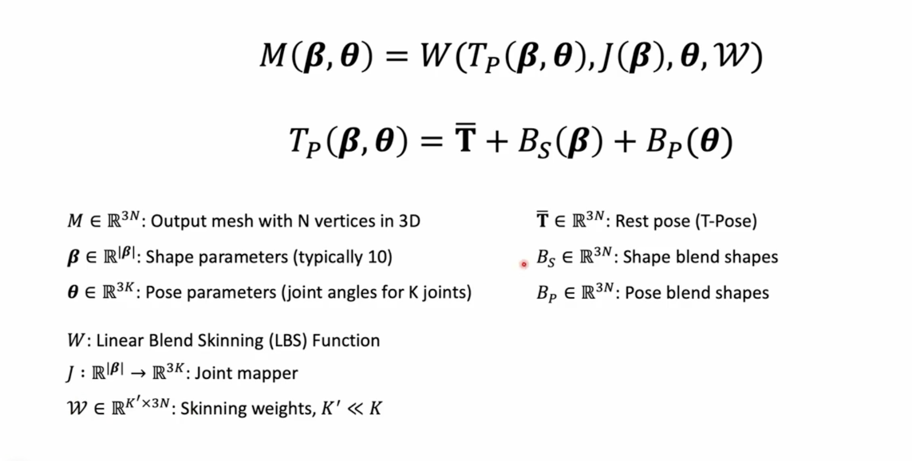
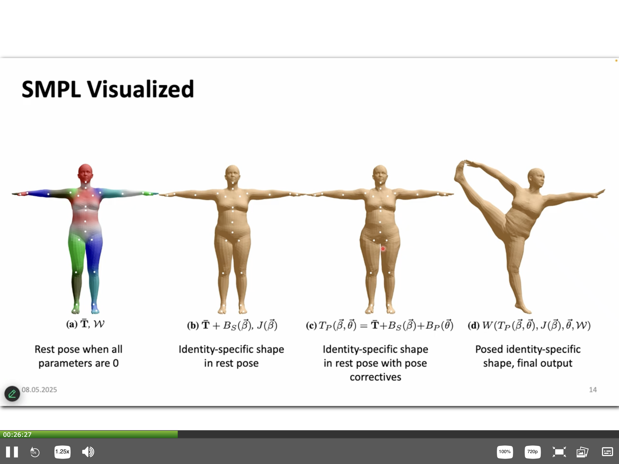
SMPL - Skinned Multi-Person Linear Model

• Description:
  • A parametric, statistical model of the human body that outputs a 3D mesh and corresponding joint locations.
  • Inputs: A vector of shape parameters (\(\beta\)) and a vector of pose parameters (\(\theta\)).
• Core Components:
  • Template Mesh (\(\bar{T}\)): A base 3D mesh with a fixed topology (standard SMPL has 6890 vertices), typically in a canonical pose (e.g., T-pose or A-pose). \(\bar{T}\) often represents the mean shape.
  • Shape Blend Shapes (\(B_S(\beta; S)\)):
    • Vertex offsets added to the template mesh to represent variations in body shape due to identity.
    • Defined as a linear combination: \[ B_S(\beta; S) = \sum_{k=1}^{|\beta|} \beta_k S_k \] where:
      • \(S_k \in \mathbb{R}^{3N}\) are orthonormal basis shapes (e.g., learned via PCA from a dataset of registered 3D scans), \(N\) is the number of vertices,
      • \(\beta_k\) are scalar shape coefficients.
    • The shaped mesh in its rest pose (before posing) is \(V_{shape} = \bar{T} + B_S(\beta; S)\).
  • Joint Locations (\(J(\beta; \mathcal{R})\)):
    • The 3D locations of \(K\) predefined joints (e.g., 23 in the basic SMPL model, plus a root) are regressed from the vertices of the shaped mesh in its rest pose: \[ J(\beta; \mathcal{R}) = \mathcal{R}(V_{shape}) \] where \(\mathcal{R}\) is a learned regressor (e.g., a linear regression matrix).
  • Pose (\(\theta\)):
    • Represents body articulation as a set of 3D rotations for each of the \(K\) joints relative to its parent in a kinematic tree structure.
    • SMPL uses an axis-angle representation for joint rotations, so \(\theta_k \in \mathbb{R}^3\) for each joint \(k\).
    • The full pose vector \(\theta \in \mathbb{R}^{(K+1) \times 3}\) includes the global orientation of the body and the relative rotations of \(K\) joints.
  • Pose Blend Shapes (\(B_P(\theta; P)\)):
    • Corrective vertex offsets added to the shaped rest mesh to mitigate artifacts from standard Linear Blend Skinning (LBS), such as joint collapse or the “candy-wrapper” effect during extreme rotations.
    • Dependent on the input pose \(\theta\). The formulation is: \[ B_P(\theta; P) = \sum_{m=1}^{9K} (R_m(\theta) - R_m(\theta^*)) P_m \] where:
      • \(R(\theta): \mathbb{R}^{(K+1) \times 3} \rightarrow \mathbb{R}^{9K}\) maps the axis-angle pose vector \(\theta\) to a vector of concatenated \(3 \times 3\) rotation matrix elements for \(K\) joints (each \(3 \times 3\) matrix has 9 elements),
      • \(R_m(\theta)\) is the \(m\)-th element of this vectorized rotation matrix representation,
      • \(\theta^*\) represents the rest pose (e.g., T-pose),
      • \(P_m \in \mathbb{R}^{3N}\) are learned pose-corrective basis displacement vectors, \(P = [P_1, ..., P_{9K}] \in \mathbb{R}^{3N \times 9K}\) is the matrix of all pose blend shape bases.
      • Subtracting \(R_m(\theta^*)\) ensures that \(B_P(\theta^*; P) = 0\), so pose blend shapes have no effect in the rest pose.
  • Linear Blend Skinning (LBS):
    • Standard algorithm in computer graphics to deform mesh vertices according to the rotations of the articulated skeleton.
    • The mesh to be deformed by LBS is the template mesh modified by both shape and pose blend shapes: \[ V_{posed\_rest} = \bar{T} + B_S(\beta; S) + B_P(\theta; P) \]
    • Each vertex \(v_i\) of \(V_{posed\_rest}\) is transformed by a weighted sum of the transformations \(G_j(\theta, J(\beta; \mathcal{R}))\) of its influencing joints: \[ v'_i = \sum_{j=0}^{K} w_{i,j} G_j(\theta, J(\beta; \mathcal{R})) v_i \] where:
      • \(v'_i\) is the final transformed vertex,
      • \(w_{i,j}\) are the skinning weights, defining the influence of joint \(j\) on vertex \(v_i\) (learned parameters in SMPL),
      • \(G_j(\theta, J(\beta; \mathcal{R}))\) is the global rigid transformation (rotation and translation) of joint \(j\) in world space, derived from the pose parameters \(\theta\) and the joint locations \(J(\beta; \mathcal{R})\) through forward kinematics.
  • Final Model Output Function:
    • The complete SMPL model \(M(\beta, \theta; \bar{T}, S, P, \mathcal{R}, W)\) generates the final posed 3D mesh vertices: \[ M(\beta, \theta) = \text{LBS}(\bar{T} + B_S(\beta; S) + B_P(\theta; P), J(\beta; \mathcal{R}), \theta, W) \]
    • The parameters to the right of the semicolon (\(\bar{T}, S, P, \mathcal{R}, W\)) are learned model parameters, while \(\beta\) and \(\theta\) are user inputs.

• Learning SMPL:
  • The model parameters (template \(\bar{T}\), shape bases \(S\), pose bases \(P\), joint regressor \(\mathcal{R}\), and skinning weights \(W\)) are learned by optimizing them to fit a large dataset of 3D body scans of different individuals in various poses.
• Challenges in Registration for Learning SMPL:
  • Aligning high-resolution, often noisy, and incomplete scan data to the SMPL template mesh topology.
  • Handling complex poses, self-contact, and smooth, featureless areas on the body surface during registration.
• Optimization during Learning:
  • Typically involves minimizing an objective function that includes data terms (e.g., Euclidean distance between registered scan vertices and corresponding model vertices) and regularization terms (e.g., to ensure smooth shapes, prevent interpenetration, enforce plausible joint limits).
  • Co-registration techniques might be employed, where model parameters and scan-to-model correspondences are optimized simultaneously or iteratively.

Human Mesh Recovery (HMR) (2018)

• Methodology:
  • Deep learning-based approach to directly regress SMPL parameters (pose \(\theta\), shape \(\beta\)) and camera parameters from a single input image.
  • The regressed parameters are then fed into the SMPL model to generate a 3D mesh.
  • Often employs an adversarial training setup:
    • A discriminator network is trained to distinguish between SMPL parameters regressed from images and those obtained from “real” 3D scan data (or mocap data), encouraging the regressor to produce more realistic and plausible body configurations.

SMPLify / SMPLify-X (SMPLify: 2016; SMPLify-X: 2019)

• Methodology:
  • Optimization-based approach to fit the SMPL model (or its extensions like SMPL-X, which includes hands and face articulation) to 2D evidence extracted from an image.
• Process:
  • Initialize SMPL parameters (e.g., to a mean pose/shape, or from an initial estimate by a regression network).
  • Iteratively optimize the pose \(\theta\) and shape \(\beta\) parameters (and potentially camera parameters, global translation) to minimize an objective function.
  • The objective function typically includes:
    • Data Term: Penalizes the discrepancy between the 2D projection of 3D SMPL joints and detected 2D keypoints in the image. Silhouettes or other cues can also be used.
    • Shape Prior: Encourages plausible body shapes, often by penalizing \(\beta\) coefficients that deviate significantly from a learned distribution (e.g., a Gaussian prior, \(\|\beta\|^2\)).
    • Pose Prior: Penalizes unnatural or impossible poses. This can be implemented using priors learned from motion capture (mocap) data, such as joint angle limits or models for interpenetration avoidance.
  • Unlike HMR, SMPLify does not directly regress parameters from image features via a deep network; instead, it relies on pre-detected 2D (or sometimes 3D) landmarks and performs an iterative optimization.

Fitting SMPL to IMU Measurements

• Methodology:
  • Utilizes data from Inertial Measurement Units (IMUs), which typically consist of accelerometers and gyroscopes, attached to various body segments.
  • IMU data provides orientation (and derivatives like angular velocity, linear acceleration) for these segments.
  • This sensor data can be used to estimate joint orientations (\(\theta\)) and subsequently fit the SMPL model, often in real-time.
  • Electromagnetic sensors can also provide positional and orientational data for similar fitting procedures.
• Challenges:
  • Sensor Drift: IMUs, particularly gyroscopes, are prone to integration drift over time, leading to orientation errors.
  • Magnetic Disturbances: Electromagnetic sensors can be affected by metallic objects or magnetic fields in the environment.
  • Sparsity: Mapping data from a sparse set of sensors to a full-body pose.
  • Calibration: Accurate sensor-to-segment calibration (aligning sensor axes with body segment coordinate systems) is crucial.

Modeling Clothing on Parametric Bodies

• Limitations of SMPL: The base SMPL model represents a minimally-clothed or naked body. Clothing is not explicitly part of its learned parameters or fixed topology.
• Approaches for Modeling Clothing on SMPL-like Bodies:
  • Displacement Maps: Learning vertex displacements from the base body surface to represent the geometry of relatively static clothing.
  • Implicit Representations:
    • Using neural implicit functions, such as Signed Distance Functions (SDFs) or occupancy fields, conditioned on body pose, shape, and potentially clothing type/style parameters to model the clothed surface.
    • Animated Neural Implicit Surfaces: A promising research direction for modeling dynamic clothed humans, where the implicit surface deforms according to body motion and learned or simulated clothing dynamics.
  • Explicit Clothed Avatars:
    • Learning separate geometric models for individual garments.
    • Combining these garment models with the body model, often involving physics-based simulation for realistic cloth behavior or data-driven deformation techniques.
• Challenges:
  • Clothing introduces significant geometric complexity and dynamic behavior (wrinkles, folds, material properties) not captured by SMPL’s fixed topology or LBS.
  • Modeling the vast diversity of clothing types, their interactions with the body, and material properties remains a complex task.