Neural Network Basics

Biological Motivation

The architecture of artificial neural networks is loosely inspired by biological neural systems.

Signal Reception and Integration: In biological neurons, dendrites receive chemical signals from other neurons. These signals are integrated in the cell body (soma).
Thresholding and Activation: If the integrated signal surpasses a certain threshold, the neuron “fires,” generating an action potential. This thresholding mechanism introduces non-linearity into the system, as the neuron only transmits a signal if the input excitation is sufficient.
Signal Transmission: The action potential travels down the axon to the axon terminals.
Synaptic Transmission: At the axon terminals, neurotransmitters are released into the synapse (the junction between two neurons), which are then received by the dendrites of a subsequent neuron, continuing the signal propagation.

Perceptron

The Perceptron, introduced by Frank Rosenblatt in 1958, is one of the earliest and simplest types of artificial neural networks, functioning as a linear classifier.

Definition: For an input vector $x$, the Perceptron computes an output $y$ based on weights $w$ and a bias $b$. The output is typically determined by whether the weighted sum $w^T x + b$ exceeds a threshold (often 0): \[ y = \begin{cases} 1 & \text{if } w^T x + b > 0 \\ 0 & \text{otherwise} \end{cases} \] This can be seen as a simple linear classifier.
Training:
- The Perceptron is typically trained using a form of gradient descent, specifically the Perceptron learning rule, which is a type of stochastic gradient descent.
- Early Perceptron models used a step activation function, resulting in binary outputs (e.g., 0 or 1, or -1 and 1). The learning rule updates weights based on misclassifications.
Capabilities and Limitations:
- If a dataset is linearly separable, the Perceptron convergence theorem guarantees that the Perceptron learning algorithm will find a separating hyperplane in a finite number of steps.
- However, the Perceptron does not necessarily find an optimal separating hyperplane (e.g., one that maximizes the margin, as Support Vector Machines do). It simply finds a solution.
- If the data is not linearly separable, the basic Perceptron algorithm may not converge.
Modern Context: Modern neural networks build upon these foundational concepts by employing multiple layers of neurons (forming “deep” networks) and using smooth, differentiable activation functions instead of the Heaviside step function. This allows for the learning of more complex, non-linear decision boundaries and the use of more sophisticated gradient-based optimization algorithms like backpropagation.

Maximum Likelihood Estimation (MLE)

Maximum Likelihood Estimation (MLE) is a fundamental statistical method used to estimate the parameters $\theta$ of a model. In the context of supervised learning, we aim to model the conditional probability $p_{\text{model}}(y | X, \theta)$, where $y$ represents the target variable(s) and $X$ represents the input features.

Likelihood Function: Assuming independent and identically distributed (i.i.d.) data samples $(x_i, y_i)$, the likelihood of observing the entire dataset $\mathcal{D} = \{(x_1, y_1), \dots, (x_N, y_N)\}$ is given by: \[ L(\theta | X, Y) = P(Y | X, \theta) = \prod_{i=1}^{N} p_{\text{model}}(y_i | x_i, \theta) \]
Log-Likelihood: It is often more convenient to work with the log-likelihood, as it converts products into sums and does not change the location of the maximum: \[ \mathcal{L}(\theta | X, Y) = \log L(\theta | X, Y) = \sum_{i=1}^{N} \log p_{\text{model}}(y_i | x_i, \theta) \] In machine learning, the negative log-likelihood (NLL) is commonly used as a loss function to be minimized: \[ \text{Loss}(\theta) = - \mathcal{L}(\theta | X, Y) = - \sum_{i=1}^{N} \log p_{\text{model}}(y_i | x_i, \theta) \]
Gradient for Optimization: To find the parameters $\theta$ that maximize the likelihood (or minimize the NLL), we typically take the derivative of the log-likelihood with respect to $\theta$, set it to zero, and solve. For complex models, iterative optimization methods like gradient descent are used:

\[ \nabla_{\theta} \mathcal{L}(\theta | X, Y) = \sum_{i=1}^{N} \nabla_{\theta} \log p_{\text{model}}(y_i | x_i, \theta) \]
- Gradient of Sigmoid Activation: For a neuron with a sigmoid activation function $\sigma(z) = \frac{1}{1 + e^{-z}}$, where $z = w^T x + b$, its derivative with respect to $z$ is: \[ \frac{d\sigma(z)}{dz} = \sigma(z)(1 - \sigma(z)) \]
- Gradient of Softmax Activation: For a softmax output layer $S(z)_j = \frac{e^{z_j}}{\sum_k e^{z_k}}$, the derivative of the $j$-th softmax output with respect to the $k$-th input $z_k$ (before softmax) is: \[ \frac{\partial S_j}{\partial z_k} = S_j (\delta_{jk} - S_k) \] where $\delta_{jk}$ is the Kronecker delta (1 if $j=k$, 0 otherwise). When combined with a cross-entropy loss, this derivative simplifies nicely.
MLE and Common Loss Functions:
- Gaussian Likelihood and Mean Squared Error (MSE): If we assume that the target variable $y$ given input $x$ follows a Gaussian distribution with mean $f(x, \theta)$ (the model’s prediction) and constant variance $\sigma^2$: \[ p_{\text{model}}(y_i | x_i, \theta) = \mathcal{N}(y_i | f(x_i, \theta), \sigma^2) = \frac{1}{\sqrt{2\pi\sigma^2}} \exp\left(-\frac{(y_i - f(x_i, \theta))^2}{2\sigma^2}\right) \] The negative log-likelihood for one sample is: \[ -\log p_{\text{model}}(y_i | x_i, \theta) = \frac{1}{2}\log(2\pi\sigma^2) + \frac{(y_i - f(x_i, \theta))^2}{2\sigma^2} \] Minimizing the sum over all samples, and ignoring constants, is equivalent to minimizing the Mean Squared Error (MSE): \[ \text{MSE} = \frac{1}{N} \sum_{i=1}^{N} (y_i - f(x_i, \theta))^2 \]
- Laplace Likelihood and Mean Absolute Error (MAE): If we assume $y$ follows a Laplace distribution with mean $f(x, \theta)$ and scale parameter $b$: \[ p_{\text{model}}(y_i | x_i, \theta) = \text{Laplace}(y_i | f(x_i, \theta), b) = \frac{1}{2b} \exp\left(-\frac{|y_i - f(x_i, \theta)|}{b}\right) \] The negative log-likelihood for one sample is: \[ -\log p_{\text{model}}(y_i | x_i, \theta) = \log(2b) + \frac{|y_i - f(x_i, \theta)|}{b} \] Minimizing the sum over all samples, and ignoring constants, is equivalent to minimizing the Mean Absolute Error (MAE): \[ \text{MAE} = \frac{1}{N} \sum_{i=1}^{N} |y_i - f(x_i, \theta)| \]
MLE and Regularization (via Maximum A Posteriori - MAP):
- If we introduce a Gaussian prior distribution over the model weights $\theta \sim \mathcal{N}(0, \alpha^2 I)$ and perform Maximum A Posteriori (MAP) estimation, this is equivalent to minimizing the NLL plus an $L_2$ regularization term (Ridge regression): \[ \hat{\theta}_{MAP} = \arg\max_{\theta} \left( \sum_{i=1}^{N} \log p_{\text{model}}(y_i | x_i, \theta) + \log p(\theta) \right) \] This leads to a loss function like: $\text{NLL} + \lambda ||\theta||_2^2$.
- If we introduce a Laplace prior over the model weights $\theta \sim \text{Laplace}(0, \beta)$ and perform MAP estimation, this is equivalent to minimizing the NLL plus an $L_1$ regularization term (Lasso regression): This leads to a loss function like: $\text{NLL} + \lambda ||\theta||_1$.
Properties of MLE:
- Consistency: MLE is consistent, meaning that as the number of samples $N$ approaches infinity, the MLE $\hat{\theta}_{MLE}$ converges in probability to the true parameter value $\theta_0$.
- Asymptotic Efficiency: MLE is asymptotically efficient. It achieves the Cramér-Rao lower bound, meaning it has the lowest possible variance among all asymptotically unbiased estimators as $N \to \infty$.
- Asymptotic Normality: Under certain regularity conditions, the distribution of $\hat{\theta}_{MLE}$ approaches a normal distribution as $N \to \infty$.

Backpropagation

Backpropagation is the cornerstone algorithm for training multi-layer neural networks. It efficiently computes the gradient of the loss function with respect to the network’s weights by applying the chain rule of calculus.

Chain Rule: For a composite function, e.g., $L(y, \hat{y})$ where $\hat{y} = f(z)$ and $z = g(W, x)$, the gradient of $L$ with respect to weights $W$ in an earlier layer is computed by propagating gradients backward from the output layer. If $L$ is the loss, $y^{(L)}$ is the output of layer $L$, $y^{(l)}$ is the output of layer $l$, and $W^{(l)}$ are the weights of layer $l$, then:

\[ \frac{\partial L}{\partial W^{(l)}} = \frac{\partial L}{\partial y^{(L)}} \frac{\partial y^{(L)}}{\partial y^{(L-1)}} \dots \frac{\partial y^{(l+1)}}{\partial y^{(l)}} \frac{\partial y^{(l)}}{\partial W^{(l)}} \]

More precisely, for a given layer $l$, the error $\delta^{(l)}$ is propagated backwards:

\[ \delta^{(l)} = ((W^{(l+1)})^T \delta^{(l+1)}) \odot \sigma'(z^{(l)}) \]

where $\sigma'$ is the derivative of the activation function at layer $l$, $z^{(l)}$ is the pre-activation output of layer $l$, and $\odot$ denotes element-wise product. The gradient with respect to weights $W^{(l)}$ is then:

\[ \frac{\partial L}{\partial W^{(l)}} = \delta^{(l)} (a^{(l-1)})^T \]

where $a^{(l-1)}$ is the activation from the previous layer.
Universal Approximation Theorem (UAT): This theorem provides a theoretical justification for the expressive power of neural networks.
- Statement (Cybenko 1989, Hornik et al. 1989): Let $\sigma : \mathbb{R} \to \mathbb{R}$ be a non-constant, bounded, and continuous activation function. Let $I_m$ denote the $m$-dimensional unit hypercube $[0,1]^m$. The space of continuous real-valued functions on $I_m$ is denoted by $C(I_m)$. Then, for any function $f \in C(I_m)$ and any $\epsilon > 0$, there exists an integer $N$ (the number of neurons in the hidden layer), real constants $v_i, b_i \in \mathbb{R}$, and real vectors $w_i \in \mathbb{R}^m$ for $i = 1, \dots, N$, such that if we define: \[ g(x) = \sum_{i=1}^{N} v_i \sigma(w_i^T x + b_i) \] then $|g(x) - f(x)| < \epsilon$ for all $x \in I_m$. (More formally, $\sup_{x \in I_m} |g(x) - f(x)| < \epsilon$.)
- Implications: In essence, the theorem states that a feed-forward neural network with a single hidden layer containing a finite number of neurons and a suitable non-linear continuous activation function can approximate any continuous function defined on a compact subset of $\mathbb{R}^m$ to an arbitrary degree of precision.
- Caveats:
  - The theorem is an existence proof; it does not specify how to find the weights $w_i, v_i$ or biases $b_i$, nor does it guarantee that they can be learned by a particular algorithm like gradient descent.
  - The number of neurons $N$ required might be very large.
  - It applies to continuous activation functions. For non-continuous ones like ReLU (Rectified Linear Unit), similar theorems exist.

Training Neural Networks

Regularization

Regularization encompasses a set of strategies designed to reduce a model’s test error (generalization error), sometimes at the cost of a slight increase in training error. The primary goal is to prevent overfitting, thereby improving the model’s performance on unseen data. Informally, these strategies often “make training harder” by constraining the model or introducing noise, compelling it to learn more robust and generalizable features.

Definition: Techniques aimed at minimizing the generalization gap (the difference between test error and training error).

Parameter Norm Penalties

These methods aim to limit the model’s effective capacity by adding a penalty term to the loss function based on the magnitude of the model parameters (weights).

L2 Regularization (Ridge Regression / Weight Decay):
- Adds a penalty proportional to the sum of the squares of the weights: $L_{reg} = \lambda ||w||_2^2 = \lambda \sum_i w_i^2$.
- This encourages smaller, more diffuse weight values.
- The gradient of this penalty term with respect to a weight $w_j$ is $2 \lambda w_j$. In the weight update rule ($w \leftarrow w - \eta (\nabla L_{data} + \nabla L_{reg})$), this results in $w_j \leftarrow w_j - \eta ( \dots + 2 \lambda w_j ) = w_j (1 - 2 \eta \lambda) - \dots$, effectively shrinking the weights by a constant factor in each step (hence “weight decay”).
L1 Regularization (Lasso):
- Adds a penalty proportional to the sum of the absolute values of the weights: $L_{reg} = \lambda ||w||_1 = \lambda \sum_i |w_i|$.
- This is known for inducing sparsity, meaning it tends to drive many weights to exactly zero, effectively performing feature selection.
- The gradient of this penalty term with respect to $w_j$ is $\lambda \text{sign}(w_j)$ (for $w_j \neq 0$). The update rule subtracts a constant value ($\eta \lambda$) from positive weights and adds it to negative weights, pushing them towards zero, irrespective of their current magnitude (as long as they are non-zero).
Interpretations:
- Bayesian Prior: Parameter norm penalties can be interpreted as imposing a prior distribution on the weights in a Maximum A Posteriori (MAP) estimation framework. L2 regularization corresponds to a Gaussian prior, while L1 regularization corresponds to a Laplace prior.
- Constrained Optimization: They are also equivalent to solving a constrained optimization problem where the weights are constrained to lie within an $L_2$ ball (for L2) or an $L_1$ ball (for L1).

Ensemble Methods

Ensemble methods combine predictions from multiple models to achieve better performance and robustness than any single constituent model.

General Idea: Train several different models and then average their predictions (for regression) or take a majority vote (for classification).
Sources of Diversity:
- Train different model architectures on the same data.
- Train the same model architecture on different subsets of the data or with different initializations.
Bagging (Bootstrap Aggregating):
- Trains multiple instances of the same base model on different bootstrap samples (random subsets of the training data, sampled with replacement).
- Primarily reduces variance and helps prevent overfitting. Random Forests are a prominent example.
Boosting:
- Trains multiple base models sequentially. Each new model focuses on correcting the errors made by the previous models (e.g., by up-weighting misclassified examples).
- Primarily reduces bias. Examples include AdaBoost, Gradient Boosting Machines (GBMs), and XGBoost.

Dropout

Dropout is a regularization technique specifically for neural networks that prevents complex co-adaptations of neurons.

Mechanism: During training, for each forward pass, a fraction of neuron outputs in a layer are randomly set to zero (dropped out). The dropout probability (e.g., $p=0.5$) is a hyperparameter.
Ensemble Interpretation: Dropout can be viewed as implicitly training a large ensemble of thinned networks (networks with different subsets of neurons).
Inference Time:
- Weight Scaling: The most common approach is to use the full network at test time, but scale down the weights of the dropout layers by the dropout probability $p$ (or, more commonly, scale up activations by $1/(1-p)$ during training – known as inverted dropout – so no scaling is needed at test time). This approximates averaging the predictions of the exponentially many thinned networks.
- Monte Carlo (MC) Dropout: Alternatively, one can perform multiple forward passes with dropout still active at test time and average the predictions. This provides an estimate of model uncertainty.

Data Normalization

Normalizing input data can stabilize and accelerate training.

Motivation: Large input values or features with vastly different scales can lead to correspondingly large weight updates and an ill-conditioned loss landscape, potentially causing training instability or slow convergence.
Common Practice: Standardize features to have zero mean and unit variance: $x'_{ij} = (x_{ij} - \mu_j) / \sigma_j$, where $\mu_j$ and $\sigma_j$ are the mean and standard deviation of feature $j$ over the training set.
Test Time: The same mean and standard deviation values computed from the training data must be used to normalize test data to prevent data leakage and ensure consistency.

Batch Normalization (BN)

Batch Normalization normalizes the activations within the network, layer by layer, to address the problem of internal covariate shift.

Mechanism:
1. For each mini-batch during training, compute the mean $\mu_{\mathcal{B}}$ and variance $\sigma_{\mathcal{B}}^2$ of the activations for each feature/channel, along the batch dimension.
2. Normalize the activations: $\hat{x}_i = (x_i - \mu_{\mathcal{B}}) / \sqrt{\sigma_{\mathcal{B}}^2 + \epsilon}$.
3. Scale and shift the normalized activations using learned parameters $\gamma$ (scale) and $\beta$ (shift): $y_i = \gamma \hat{x}_i + \beta$. These parameters allow the network to learn the optimal distribution for activations, potentially undoing the normalization if necessary.
Inference Time: During inference, the mini-batch statistics are unavailable. Instead, population statistics (running means and variances) estimated during training (e.g., via exponential moving averages of mini-batch means/variances) are used for normalization.
Benefits:
- Reduces internal covariate shift (changes in the distribution of layer inputs during training), stabilizing learning.
- Allows for higher learning rates and can make training less sensitive to weight initialization.
- The bias terms in layers preceding BN become redundant (as $\beta$ can fulfill their role) and can often be omitted.
- The stochasticity introduced by using mini-batch statistics for normalization has a slight regularization effect.

Data Augmentation

Data augmentation artificially expands the training dataset by creating modified copies of existing data or synthesizing new data.

Principle: More diverse training data generally leads to better generalization and robustness.
Technique: Apply transformations to input data while preserving their labels.
Examples for Images:
- Geometric Transformations: Rotation, scaling, translation, shearing, flipping.
- Color Jittering: Adjusting brightness, contrast, saturation, hue.
Noise Injection: Adding random noise (e.g., Gaussian noise) to inputs can enforce robustness against small perturbations.

Transfer Learning

Transfer learning leverages knowledge gained from solving one problem to improve performance on a different but related problem.

Process:
1. Pre-training: A model is trained on a large-scale dataset (e.g., ImageNet for computer vision tasks). This model learns general-purpose features.
2. Fine-tuning: The pre-trained model (or parts of it) is then adapted to a smaller, target dataset. This typically involves replacing the final classification layer and re-training some or all of the network’s layers with a smaller learning rate.
Using Pre-trained Models: One can directly use well-known architectures (e.g., ResNet, VGG, BERT) that have been pre-trained on extensive datasets, saving significant training time and resources.

Activation Functions

Activation functions introduce non-linearities into the network, enabling it to learn complex patterns.

Sigmoid: $f(x) = 1 / (1 + e^{-x})$
- Output range: $(0, 1)$.
- Saturates for large positive or negative inputs, leading to vanishing gradients (gradients close to zero), which can slow down or stall learning in deep networks.
- Not zero-centered, which can be a minor issue for gradient updates.
Tanh (Hyperbolic Tangent): $f(x) = (e^x - e^{-x}) / (e^x + e^{-x})$
- Output range: $(-1, 1)$.
- Zero-centered, which is generally preferred over Sigmoid.
- Also saturates and suffers from vanishing gradients, though its gradients are typically larger than Sigmoid’s around zero.
ReLU (Rectified Linear Unit): $f(x) = \max(0, x)$
- Non-saturating in the positive domain, which helps alleviate the vanishing gradient problem and accelerates convergence.
- Computationally efficient.
- Can lead to “dead neurons”: if a neuron’s input is consistently negative, it will always output zero, and its gradient will also be zero, preventing weight updates for that neuron.
- Unbounded in the positive direction.
Leaky ReLU (LReLU) / Parametric ReLU (PReLU): $f(x) = \max(\alpha x, x)$
- Addresses the dead neuron problem by allowing a small, non-zero gradient when the unit is not active (e.g., $\alpha = 0.01$ for LReLU).
- In PReLU, $\alpha$ is a learnable parameter.
- Randomized Leaky ReLU (RReLU) samples $\alpha$ from a distribution during training.
GELU (Gaussian Error Linear Unit): $f(x) = x \Phi(x)$, where $\Phi(x)$ is the cumulative distribution function (CDF) of the standard Gaussian distribution.
- A smooth approximation of ReLU, often performing well in Transformer models.
- Approximation: $f(x) \approx 0.5x (1 + \tanh[\sqrt{2/\pi}(x + 0.044715x^3)])$.
- Non-saturating in the positive domain.
Initialization: Proper weight initialization techniques (e.g., He initialization for ReLU-like activations) can also help mitigate issues like dead neurons and improve training stability.

Optimization Algorithms

Optimization algorithms adjust the model’s parameters (weights and biases) to minimize the loss function.

Gradient Descent Variants:
- Batch Gradient Descent (Full GD): Computes the gradient using the entire training dataset. Accurate but computationally expensive for large datasets and can get stuck in local minima.
- Stochastic Gradient Descent (SGD): Computes the gradient using a single training example at a time. Faster updates, noisy gradients can help escape local minima, but high variance in updates.
- Mini-Batch Gradient Descent: Computes the gradient using a small batch of training examples. Strikes a balance between the accuracy of full GD and the efficiency/stochasticity of SGD. This is the most common approach.

Momentum-Based Methods

These methods accelerate SGD by incorporating information from past updates.

Polyak’s Momentum (Heavy Ball Method):
- Addresses oscillations in SGD, particularly in ravines (areas where the surface curves more steeply in one dimension than another).
- Maintains an exponentially moving average (EMA) of past gradients, which acts as a “velocity” term.
- Update equations: Let $g_t = \nabla_{\theta} J(\theta_t)$ be the gradient at time $t$. Velocity (EMA of gradients): $v_t = \beta v_{t-1} + (1 - \beta) g_t$ Parameter update: $\theta_{t+1} = \theta_t - \eta v_t$ where $\beta$ is the momentum coefficient (e.g., 0.9) and $\eta$ is the learning rate.
- Convergence: While standard SGD with momentum is widely used and effective for non-convex optimization, its convergence properties can be complex. Polyak’s original heavy ball method has convergence guarantees for strongly convex functions.
Nesterov Accelerated Gradient (NAG):
- A modification of momentum that provides a “lookahead” capability. It calculates the gradient not at the current position $\theta_t$, but at an approximated future position $\theta_t - \eta \beta v_{t-1}$ (where the parameters would be after applying the previous momentum). This allows for a more informed gradient step.
- Update equations (one common formulation): Lookahead point: $\theta_{lookahead} = \theta_t - \eta_{lr} \beta v_{t-1}$ Gradient at lookahead: $g_{lookahead} = \nabla J(\theta_{lookahead})$ Velocity EMA: $v_t = \beta v_{t-1} + (1-\beta) g_{lookahead}$ Parameter update: $\theta_{t+1} = \theta_t - \eta_{lr} v_t$
- Alternatively, a common implementation form (e.g., Hinton et al.): $v_{t+1} = \mu v_t - \epsilon \nabla J(\theta_t + \mu v_t)$ $\theta_{t+1} = \theta_t + v_{t+1}$ where $\mu$ is momentum and $\epsilon$ is learning rate.
- The “lookahead” often provides faster convergence and better performance than standard momentum. The computation of gradients at different points can be re-written through a change of variables for implementation.

Adaptive Learning Rate Methods

These methods adjust the learning rate for each parameter individually based on the history of gradients.

Adagrad (Adaptive Gradient Algorithm):
- Adapts the learning rate for each parameter, performing larger updates for infrequent parameters and smaller updates for frequent parameters.
- Accumulates the sum of squared past gradients for each parameter.
- Update for parameter $\theta_i$: \[ G_{t,ii} = G_{t-1,ii} + g_{t,i}^2 \] \[ \theta_{t+1, i} = \theta_{t, i} - \frac{\eta}{\sqrt{G_{t,ii} + \epsilon}} g_{t,i} \] where $g_{t,i}$ is the gradient of the loss with respect to $\theta_i$ at time $t$, $G_t$ is a diagonal matrix where each diagonal element $G_{t,ii}$ is the sum of squares of past gradients for $\theta_i$, $\eta$ is a global learning rate, and $\epsilon$ is a small constant for numerical stability.
- Strength: Good for sparse data.
- Weakness: The learning rate monotonically decreases and can become too small prematurely, effectively stopping learning.
RMSProp (Root Mean Square Propagation):
- Addresses Adagrad’s aggressively diminishing learning rates by using an exponentially decaying moving average of squared gradients instead of summing all past squared gradients.
- Update for parameter $\theta_i$: \[ E[g^2]_{t,i} = \gamma E[g^2]_{t-1,i} + (1-\gamma) g_{t,i}^2 \] \[ \theta_{t+1, i} = \theta_{t, i} - \frac{\eta}{\sqrt{E[g^2]_{t,i} + \epsilon}} g_{t,i} \] where $E[g^2]_{t,i}$ is the moving average of squared gradients for $\theta_i$, and $\gamma$ is the decay rate (e.g., 0.9).
Adam (Adaptive Moment Estimation):
- Combines the ideas of momentum (using an EMA of past gradients, first moment) and adaptive learning rates (using an EMA of past squared gradients, second moment, similar to RMSProp).
- Includes bias correction terms for the first and second moment estimates, which are particularly important during the initial stages of training when the EMAs are initialized at zero.
- Update equations: $m_t = \beta_1 m_{t-1} + (1-\beta_1) g_t$ (EMA of gradients - 1st moment) $v_t = \beta_2 v_{t-1} + (1-\beta_2) g_t^2$ (EMA of squared gradients - 2nd moment) Bias-corrected estimates: \[ \hat{m}_t = \frac{m_t}{1 - \beta_1^t} \] \[ \hat{v}_t = \frac{v_t}{1 - \beta_2^t} \] Parameter update: \[ \theta_{t+1} = \theta_t - \frac{\eta}{\sqrt{\hat{v}_t} + \epsilon} \hat{m}_t \] where $\beta_1$ (e.g., 0.9) and $\beta_2$ (e.g., 0.999) are decay rates for the moment estimates. Adam is often a good default choice for many problems.

Learning Rate Schedules

A learning rate schedule dynamically adjusts the learning rate during training.

Step Decay: Reduces the learning rate by a fixed factor (e.g., 0.1) every few epochs.
Exponential Decay: Reduces the learning rate exponentially: $\eta_t = \eta_0 \exp(-kt)$, where $k$ is a decay rate.
Time-Based Decay: Reduces the learning rate as a function of iteration number, e.g., $\eta_t = \eta_0 / (1 + kt)$.
Cosine Annealing: Varies the learning rate according to a cosine function, typically from an initial high value $\eta_{max}$ down to a minimum value $\eta_{min}$ (often 0) over a specified number of epochs (a “cycle”). \[ \eta_t = \eta_{min} + \frac{1}{2}(\eta_{max} - \eta_{min})\left(1 + \cos\left(\frac{T_{cur}}{T_{cycle}}\pi\right)\right) \] where $T_{cur}$ is the current epoch/iteration within the cycle and $T_{cycle}$ is the total duration of the cycle. This schedule smoothly decreases the learning rate. It can be used with “restarts” (SGDR - Stochastic Gradient Descent with Warm Restarts), where the cosine cycle is repeated multiple times.

Advanced Ensemble and Weight Averaging Techniques

Beyond basic bagging and boosting, several techniques leverage model weights or training dynamics for ensembling.

Snapshot Ensembling: Train a single model, but save “snapshots” (checkpoints) of its weights at different points during training (often at local minima found by a cyclical learning rate schedule). These snapshots are then ensembled.
Polyak-Ruppert Averaging (or EMA of weights): Maintain an exponential moving average of the model’s weights during the later stages of training. This averaged model often generalizes better.

Fast Geometric Ensembling (FGE)

FGE leverages the observation that local minima in the loss landscape of deep neural networks are often connected by simple, low-loss paths.

Concept: Train a single network using a cyclical learning rate schedule (e.g., multiple cycles of cosine annealing).
Procedure:
1. Define a learning rate schedule with multiple cycles (e.g., $M$ cycles over $T$ total epochs). Each cycle involves a period of higher learning rate followed by a decrease to a very low learning rate.
2. At the end of each cycle, when the learning rate is at its minimum (allowing the model to converge to a local optimum), save a snapshot of the model weights.
3. The ensemble consists of these $M$ saved models. Their predictions are averaged at inference time.
Benefit: Allows finding multiple diverse, high-performing models with roughly the same computational cost as training a single model.

Stochastic Weight Averaging (SWA)

SWA is a simpler approximation that often yields similar benefits to FGE, leading to wider optima and better generalization.

Procedure:
1. Initial Training: Train a model using a standard learning rate schedule for a certain number of epochs (e.g., 75% of the total training budget).
2. SWA Phase: For the remaining epochs (e.g., 25%), switch to a modified learning rate schedule:
  - Typically a constant high learning rate or a cyclical schedule with a relatively high average (e.g., short cosine annealing cycles).
3. Weight Collection: During this SWA phase, collect model weights at regular intervals (e.g., at the end of each epoch or every few iterations).
4. Averaging: Compute the average of these collected weights: $w_{SWA} = \frac{1}{N_{models}} \sum_{i=1}^{N_{models}} w_i$.
5. Batch Normalization Update: After obtaining $w_{SWA}$, perform a forward pass over the entire training data using the $w_{SWA}$ model to recompute the Batch Normalization running statistics. This is crucial for good performance.
Inference: Use the $w_{SWA}$ model for predictions.
Advantages: Easy to implement and often provides a significant performance boost with minimal additional computational cost beyond the initial training.

Convolutional Neural Networks (CNNs)

Convolutional Neural Networks (CNNs) are a class of deep neural networks particularly well-suited for processing grid-like data, such as images.

Wide Range of Applications:
- Image classification, object localization, instance segmentation, semantic segmentation, 3D pose estimation, eye gaze estimation, dynamic gesture recognition, and more.
Biological Inspiration:
- CNNs are inspired by the organization of the animal visual cortex.
- Hubel and Wiesel (1950s-1960s) discovered a hierarchy in the visual cortex:
  - Simple cells: Respond to specific features (e.g., oriented edges) at particular locations; susceptible to noise.
  - Complex cells: Aggregate responses from simple cells, providing spatial invariance and robustness.
Neocognitron (Fukushima, 1980):
- Early hierarchical neural network model for visual pattern recognition.
- S-cells: Simple cells, analogous to convolutional filters.
- C-cells: Complex cells, analogous to pooling layers.

The Convolution Operation in CNNs

Properties:
- Linear transformation.
- Shift equivariance: Shifting the input shifts the output in the same way.
Mathematical Definition (Convolution):
- Given input image $I$ and kernel $K$, the output $I'$ is: \[ I'(i, j) = \sum_{m} \sum_{n} K(m, n) \, I(i - m, j - n) \]
Cross-Correlation (as used in most deep learning libraries): \[ I'(i, j) = \sum_{m} \sum_{n} K(m, n) \, I(i + m, j + n) \]
- True convolution is cross-correlation with a 180-degree rotated kernel: $I * K = I \star K_{\text{flipped}}$, where $K_{\text{flipped}}(m, n) = K(-m, -n)$.
Commutativity: Convolution is commutative ($I * K = K * I$), cross-correlation is not.

CNN Architecture Overview

A typical CNN consists of:

Convolutional layers: Learn spatial features.
Activation functions: Non-linearities (e.g., ReLU, sigmoid, tanh).
Pooling layers: Downsample feature maps.
Fully connected layers: Used at the end for classification/regression.

Mathematical Derivation of a Convolutional Layer

Let $z^{[l-1]}_{u, v}$ be the output of layer $l-1$ at position $(u, v)$. Let $w^{[l]}_{m, n}$ be the filter weights, and $b^{[l]}$ the bias.

Forward Pass:

\[ z^{[l]}_{i, j} = \sum_{m} \sum_{n} w^{[l]}_{m, n} \, z^{[l-1]}_{i - m, j - n} + b^{[l]} \]

Backward Pass:

Let $L$ be the loss, and $\delta^{[l]}_{i, j} = \frac{\partial L}{\partial z^{[l]}_{i, j}}$.

Gradient w.r.t. previous layer activations:

\[ \delta^{[l-1]}_{i, j} = \sum_{m} \sum_{n} \delta^{[l]}_{i + m, j + n} \, w^{[l]}_{m, n} \]
- This is equivalent to convolving $\delta^{[l]}$ with the kernel $w^{[l]}$ rotated by 180 degrees: \[ \delta^{[l-1]} = \delta^{[l]} * \text{rot180}(w^{[l]}) \]
Gradient w.r.t. weights:

\[ \frac{\partial L}{\partial w^{[l]}_{m, n}} = \sum_{i} \sum_{j} \delta^{[l]}_{i, j} \, z^{[l-1]}_{i - m, j - n} \]
- This is the cross-correlation of $z^{[l-1]}$ with $\delta^{[l]}$.
Gradient w.r.t. bias: \[ \frac{\partial L}{\partial b^{[l]}} = \sum_{i} \sum_{j} \delta^{[l]}_{i, j} \]

Pooling Layers

Purpose: Downsample feature maps, reduce computation, and provide translation invariance.
Max pooling: Takes the maximum value in a local region.
- No parameters.
- During backpropagation, the gradient is passed only to the input that had the maximum value.
Average pooling: Takes the average value in a local region.
Modern trend: Strided convolutions often replace pooling.

Convolution and Cross-Correlation Identities

$A * \text{rot180}(B) = A \star B$
$A \star B = \text{rot180}(B) * A$

Fully Convolutional Networks (FCNs)

Semantic segmentation: Classify each pixel.
Input and output dimensions: Typically the same.
Architecture: Downsample (encoder), then upsample (decoder).
Upsampling methods:
- Fixed: Nearest neighbor, “bed of nails”, max unpooling.
- Learnable: Transposed convolution.

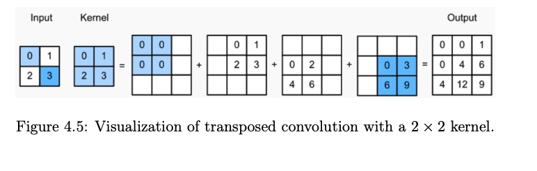
Transposed Convolution

Also called: Fractionally strided convolution, “deconvolution” (not a true inverse).
Mechanism:
- Upsample by inserting zeros between input elements.
- Apply a standard convolution to the upsampled input.
- Output size for input height $H_{in}$, kernel size $k$, stride $s$, and padding $p$: \[ H_{out} = s (H_{in} - 1) + k - 2p \]
Visualization: Each input value is multiplied by the kernel and “spread” over the output, overlapping values are summed.

U-Net Architecture

Symmetric encoder-decoder: Contracting path (encoder) for context, expanding path (decoder) for localization.
Skip connections: Concatenate encoder features with decoder features at corresponding resolutions for better localization.
Applications: Semantic segmentation, image generation from segmentation maps, 3D human pose/shape estimation, and more.

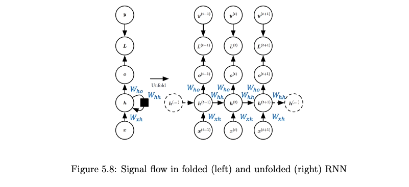
Recurrent Neural Networks (RNNs)

Recurrent Neural Networks (RNNs) are a class of artificial neural networks designed specifically for processing sequential data. Unlike feedforward neural networks, RNNs possess internal memory (state) that allows them to capture temporal dependencies and patterns over time.

Key Characteristics:
- Sequential Data Processing: Suited for tasks where the order of input elements matters, such as time series, natural language, speech, and video.
- Variable-Length Sequences: Can naturally handle input and output sequences of varying lengths.
- Internal State (Memory): Maintain a hidden state $h^t$ that is updated at each time step, summarizing information from past inputs in the sequence. This state is recurrently fed back into the network.
- Weight Sharing: The same set of weights is used across all time steps for processing different elements of the sequence. This allows the model to generalize to sequences of different lengths and learn patterns that are consistent across time.
Common RNN Architectures based on Input/Output Mapping:
- One-to-One: Standard feedforward neural network (not typically considered an RNN in this context, but serves as a baseline).
  - Example: Image classification (single input, single output).
- One-to-Many: A single input generates a sequence of outputs.
  - Example: Image captioning (input: image; output: sequence of words).
  - Example: Music generation from a seed note.
- Many-to-One: A sequence of inputs generates a single output.
  - Example: Sentiment analysis (input: sequence of words; output: sentiment label).
  - Example: Sequence classification (e.g., classifying a video based on its frames).
- Many-to-Many (Synchronous): A sequence of inputs generates a corresponding sequence of outputs, with alignment between input and output at each step.
  - Example: Video frame classification (classifying each frame in a video).
  - Example: Part-of-speech tagging (tagging each word in a sentence).
- Many-to-Many (Asynchronous/Delayed): A sequence of inputs generates a sequence of outputs, but the lengths may differ, and alignment is not necessarily one-to-one at each step.
  - Example: Machine translation (input: sentence in one language; output: sentence in another language).
  - Example: Speech recognition (input: audio sequence; output: sequence of words).

RNNs as Dynamical Systems

RNNs can be viewed as discrete-time dynamical systems.

Dynamical System Definition: A mathematical model describing the temporal evolution of a system’s state. The state at a given time is a function of its previous state and any external inputs.
- Continuous-time dynamical systems are often described by differential equations (e.g., $\frac{dh(t)}{dt} = f(h(t), x(t))$).
- RNNs are discrete-time dynamical systems, where the state $h^t$ evolves at discrete time steps $t$. The evolution is defined by a recurrence relation: \[ h^t = f(h^{t-1}, x^t; \theta) \] where $h^t$ is the hidden state at time $t$, $h^{t-1}$ is the hidden state at the previous time step, $x^t$ is the input at time $t$, and $\theta$ represents the model parameters (weights and biases).
- Relation to Hidden Markov Models (HMMs): While both RNNs and HMMs model sequences and have hidden states, they are different concepts. HMMs are probabilistic graphical models with discrete states and explicit transition/emission probabilities. RNNs are connectionist models with continuous hidden states and learn transitions implicitly through neural network functions. HMMs are a specific type of dynamical system, but not all discrete dynamical systems are HMMs.

Vanilla RNN

The “vanilla” RNN is the simplest form of a recurrent network.

State Update Equation: The hidden state $h^t$ is computed as a non-linear function of the previous hidden state $h^{t-1}$ and the current input $x^t$:

\[ h^t = \tanh(W_{hh} h^{t-1} + W_{xh} x^t + b_h) \]

where:
- $x^t$ is the input vector at time step $t$.
- $h^{t-1}$ is the hidden state vector from the previous time step $t-1$.
- $W_{xh}$ is the weight matrix connecting the input to the hidden layer.
- $W_{hh}$ is the weight matrix connecting the previous hidden state to the current hidden state (the recurrent weights).
- $b_h$ is the bias vector for the hidden layer.
- $\tanh$ is the hyperbolic tangent activation function.
Output Equation: The output $\hat{y}^t$ at time step $t$ is typically computed from the current hidden state:

\[ \hat{y}^t = W_{hy} h^t + b_y \]

where:
- $W_{hy}$ is the weight matrix connecting the hidden layer to the output layer.
- $b_y$ is the bias vector for the output layer.
Weight Sharing: The weight matrices ($W_{xh}, W_{hh}, W_{hy}$) and biases ($b_h, b_y$) are shared across all time steps.

Training: Backpropagation Through Time (BPTT)
- BPTT unrolls the RNN through time for a sequence of length $S$ and applies backpropagation.
- The total loss $L$ is the sum of losses $L^t$ at each time step (e.g., $L^t = \|\hat{y}^t - y^t\|^2$).
- The gradient of the total loss $L$ with respect to any weight matrix $W$ is: \[ \frac{\partial L}{\partial W} = \sum_{t=1}^{S} \frac{\partial L^t}{\partial W} \]
- The gradient of the loss at a specific time step $t$, $L^t$, with respect to $W$ is found by summing influences through all intermediate hidden states $h^k$: \[ \frac{\partial L^t}{\partial W} = \sum_{k=1}^{t} \frac{\partial L^t}{\partial \hat{y}^t} \frac{\partial \hat{y}^t}{\partial h^t} \frac{\partial h^t}{\partial h^k} \frac{\partial^+ h^k}{\partial W} \] where $\frac{\partial^+ h^k}{\partial W}$ is the “immediate” partial derivative.
- Vanishing/Exploding Gradients: The term $\frac{\partial h^t}{\partial h^k}$ is critical: \[ \frac{\partial h^t}{\partial h^k} = \prod_{i=k+1}^{t} \frac{\partial h^i}{\partial h^{i-1}} \] Given the state update $h^i = \tanh(W_{hh} h^{i-1} + W_{xh} x^i + b_h)$, the Jacobian is: \[ \frac{\partial h^i}{\partial h^{i-1}} = W_{hh} \operatorname{diag}(1 - (h^{i-1})^2) \] where $\operatorname{diag}(1 - (h^{i-1})^2)$ is a diagonal matrix with entries $1 - (h^{i-1}_j)^2$. Thus, the product becomes: \[ \frac{\partial h^t}{\partial h^k} = \prod_{i=k+1}^{t} \left( W_{hh} \operatorname{diag}(1 - (h^{i-1})^2) \right) \] This product involves repeated multiplication of $W_{hh}$ (and diagonal matrices).
  - If the magnitudes of eigenvalues/singular values of $W_{hh}$ are consistently greater than 1, the norm of this product can grow exponentially with $t-k$, leading to exploding gradients.
  - If they are consistently less than 1, the norm can shrink exponentially, leading to vanishing gradients.

Long Short-Term Memory (LSTM)

LSTMs were introduced by Sepp Hochreiter and Jürgen Schmidhuber in 1997 to address the vanishing gradient problem in vanilla RNNs. They achieve this through a more complex internal cell structure involving gating mechanisms.

Core Idea: LSTMs use gates (input, forget, output) to control the flow of information into and out of a cell state $c_t$. The cell state acts as a memory conveyor belt, allowing information to propagate over long durations with minimal decay.

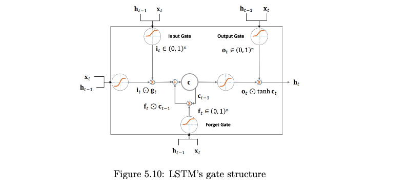
Matrix Representation for Gates and Cell Update: Let $x_t$ be the current input and $h_{t-1}$ be the previous hidden state. The core computations for the gates (forget $f_t$, input $i_t$, output $o_t$) and the candidate cell state $\tilde{c}_t$ can be combined:

\[ \begin{pmatrix} i_t \\ f_t \\ o_t \\ \tilde{c}_t \end{pmatrix} = \begin{pmatrix} \sigma \\ \sigma \\ \sigma \\ \tanh \end{pmatrix} \left( W \begin{bmatrix} x_t \\ h_{t-1} \end{bmatrix} + b \right) \]

where $W$ is a block weight matrix and $b$ is a block bias vector. The cell state $c_t$ and hidden state $h_t$ are then updated:

\[ c_t = f_t \odot c_{t-1} + i_t \odot \tilde{c}_t \]

\[ h_t = o_t \odot \tanh(c_t) \]

where $\sigma$ is the sigmoid function, $\tanh$ is the hyperbolic tangent function, and $\odot$ denotes element-wise multiplication.
Stacked LSTMs (Multiple Layers): LSTMs can be stacked to create deeper recurrent networks. The hidden state $h_t^{[l]}$ of layer $l$ at time $t$ becomes the input $x_t^{[l+1]}$ for layer $l+1$ at the same time step $t$.

Gated Recurrent Unit (GRU)

The Gated Recurrent Unit (GRU), introduced by Cho et al. in 2014, is a variation of the LSTM with a simpler architecture and fewer parameters. It often performs comparably to LSTMs on many tasks.

Key Differences from LSTM:
- It combines the forget and input gates of an LSTM into a single update gate.
- It merges the cell state and hidden state, resulting in only one state vector being passed between time steps.
- It uses a reset gate to control how much of the previous state information is incorporated into the candidate state.
GRUs are generally computationally slightly more efficient than LSTMs due to having fewer gates and parameters. The choice between LSTM and GRU often depends on the specific dataset and task, with empirical evaluation being the best guide.

Gradient Clipping

Gradient clipping is a common technique used during the training of RNNs (and other deep networks) to mitigate the exploding gradient problem.

Mechanism:
- If the L2 norm of the gradient vector $g = \frac{\partial L}{\partial W}$ (where $W$ represents all parameters, or parameters of a specific layer) exceeds a predefined threshold $\tau$, the gradient is scaled down to have a norm equal to $\tau$.
- If $\|g\|_2 > \tau$, then $g \leftarrow \frac{\tau}{\|g\|_2} g$.
- If $\|g\|_2 \le \tau$, then $g$ remains unchanged.
Purpose: It prevents excessively large gradient updates that can destabilize the training process, without changing the direction of the gradient. It does not directly solve the vanishing gradient problem.

Generative Models

The primary objective of generative modeling is to learn the underlying probability distribution $p(\text{data})$ of a dataset—either explicitly or implicitly—so that we can sample new data points from it.
- Implicit Models: Define a stochastic procedure to generate samples without an explicit density.
  - Examples: Generative Adversarial Networks (GANs), Markov Chains.
- Explicit Models: Specify a parametric form for the density $p(\text{data})$.
  - Tractable Explicit Models: The density can be evaluated directly.
    - Examples: Autoregressive models (PixelRNN, PixelCNN), Normalizing Flows.
  - Approximate Explicit Models: The density is intractable; use approximations.
    - Examples: Variational Autoencoders (VAEs), Boltzmann Machines (via MCMC).

Autoencoders (AEs)

Autoencoders are neural networks for unsupervised representation learning and dimensionality reduction.
- Encoder $f_{\phi}$: maps $x$ to latent $z = f_{\phi}(x)$.
- Decoder $g_{\theta}$: reconstructs $\hat{x} = g_{\theta}(z)$ from $z$.
- Assumes data lie on a low-dimensional manifold embedded in the input space.
- Desirable latent properties:
  - Smoothness: small changes in $z$ yield small, meaningful changes in $\hat{x}$.
  - Disentanglement: each dimension of $z$ corresponds to a distinct factor of variation.
PCA as a Linear Autoencoder: PCA minimizes $L_2$ reconstruction loss under orthonormality constraints.
Nonlinear Autoencoders: Use neural nets, optimize $\|x - \hat{x}\|_2^2$ (MSE).
Latent Dimension:
- Undercomplete: $\dim(Z) < \dim(X)$ for compression.
- Overcomplete: $\dim(Z) \ge \dim(X)$ (e.g. denoising, sparse coding).
  - Denoising Autoencoders: Train to reconstruct clean $x$ from corrupted $x'$, loss computed on $x$.
Limitation: Standard AEs lack a structured latent space; sampling arbitrary $z$ often yields poor outputs.

Variational Autoencoders (VAEs)

VAEs learn a continuous, structured latent space suitable for generation.
Encoder (Recognition Model) $q_{\phi}(z|x)$:
- Outputs parameters of a Gaussian: mean $\mu_{\phi}(x)$ and log-variance $\log \sigma^2_{\phi}(x)$.
- Defines $q_{\phi}(z|x) = \mathcal{N}(z; \mu_{\phi}(x), \mathrm{diag}(\sigma^2_{\phi}(x)))$.
Reparameterization Trick:
- Sample $\epsilon \sim \mathcal{N}(0,I)$.
- Set $z = \mu_{\phi}(x) + \sigma_{\phi}(x)\odot \epsilon$, permitting backpropagation.
Regularization & Posterior Collapse:
- Without regularization, $\sigma_{\phi}(x)\to 0$ → AE collapse.
- Posterior collapse: decoder ignores $z$.
- Remedy: add $D_{KL}(q_{\phi}(z|x)\|p(z))$ to the loss, where $p(z)=\mathcal{N}(0,I)$.
Derivation of the Objective Function (Evidence Lower Bound - ELBO):
- Goal: maximize the marginal likelihood \[ p_{\theta}(x) = \int p_{\theta}(x,z)\,dz. \]
- Insert approximate posterior $q_{\phi}(z|x)$: \[ \log p_{\theta}(x) = \log \int q_{\phi}(z|x)\,\frac{p_{\theta}(x,z)}{q_{\phi}(z|x)}\,dz = \log \mathbb{E}_{q_{\phi}(z|x)}\Bigl[\tfrac{p_{\theta}(x,z)}{q_{\phi}(z|x)}\Bigr]. \]
- Apply Jensen’s inequality ($\log$ concave): \[ \log p_{\theta}(x) \;\ge\; \mathbb{E}_{q_{\phi}(z|x)}\Bigl[\log\tfrac{p_{\theta}(x,z)}{q_{\phi}(z|x)}\Bigr]. \]
- Decompose the expectation: \[ \mathbb{E}_{q_{\phi}(z|x)}\Bigl[\log\tfrac{p_{\theta}(x,z)}{q_{\phi}(z|x)}\Bigr] = \mathbb{E}_{q_{\phi}(z|x)}[\log p_{\theta}(x|z)] + \mathbb{E}_{q_{\phi}(z|x)}[\log p(z)] - \mathbb{E}_{q_{\phi}(z|x)}[\log q_{\phi}(z|x)]. \]
- Recognize \[ \mathbb{E}_{q_{\phi}(z|x)}[\log p(z)] - \mathbb{E}_{q_{\phi}(z|x)}[\log q_{\phi}(z|x)] = -D_{KL}\bigl(q_{\phi}(z|x)\|p(z)\bigr). \]
- Therefore, \[ \log p_{\theta}(x) = \underbrace{\mathbb{E}_{q_{\phi}(z|x)}[\log p_{\theta}(x|z)]}_{(1)\,\text{Reconstruction}} \;-\;\underbrace{D_{KL}\bigl(q_{\phi}(z|x)\|p(z)\bigr)}_{(2)\,\text{Prior matching}} \;+\;\underbrace{D_{KL}\bigl(q_{\phi}(z|x)\|p_{\theta}(z|x)\bigr)}_{(3)\,\ge0\,,\text{+gap}}. \]
- The ELBO is terms (1) and (2): \[ \mathrm{ELBO}(\phi,\theta;x) = \mathbb{E}_{q_{\phi}(z|x)}[\log p_{\theta}(x|z)] - D_{KL}\bigl(q_{\phi}(z|x)\|p(z)\bigr). \]
- Maximizing the ELBO maximizes a lower bound on $\log p_{\theta}(x)$.
- The VAE loss (to minimize) is the negative ELBO: \[ L_{VAE}(\phi,\theta;x) = -\mathbb{E}_{q_{\phi}(z|x)}[\log p_{\theta}(x|z)] + D_{KL}\bigl(q_{\phi}(z|x)\|p(z)\bigr). \]
Analytical KL Divergence:
- If $q_{\phi}(z|x)=\mathcal{N}(z;\mu_{\phi}(x),\mathrm{diag}(\sigma^2_{\phi}(x)))$ and $p(z)=\mathcal{N}(0,I)$, then \[ D_{KL}\bigl(q_{\phi}(z|x)\|p(z)\bigr) = \tfrac{1}{2}\sum_{j=1}^{D}\bigl(\sigma_j^2(x)+\mu_j^2(x) -\log\sigma_j^2(x)-1\bigr). \]
Generation After Training:
- Sample $z\sim p(z)$ and decode via $p_{\theta}(x|z)$.
- Without conditioning, attributes (e.g. class) are uncontrolled.
- Conditional VAEs (CVAEs): condition on labels $y$, use $q_{\phi}(z|x,y)$ and $p_{\theta}(x|z,y)$ for controlled generation.

β-VAEs

β-VAEs introduce a hyperparameter β (>1) to the ELBO: \[ L_{\beta\text{-VAE}}(\phi,\theta;x) = -\mathbb{E}_{q_{\phi}(z|x)}[\log p_{\theta}(x|z)] + \beta\,D_{KL}\bigl(q_{\phi}(z|x)\|p(z)\bigr). \]
Rationale for Disentanglement:
- The KL term matches $q_{\phi}(z|x)$ to an isotropic Gaussian $p(z)=\mathcal{N}(0,I)$.
- Isotropy implies zero mean, unit variance, and independence across latent dimensions.
- By upweighting the KL term (β>1), β-VAEs more strongly penalize any deviation from:
  - unit variance in each $z_j$,
  - zero covariance between distinct latent axes.
- This stronger pressure reduces correlations among latent dimensions, encouraging each $z_j$ to capture an independent factor of variation.
Constrained Optimization Perspective:
- Maximizing ELBO subject to $D_{KL}(q_{\phi}(z|x)\|p(z))\le \epsilon_0$.
- β acts as a Lagrange multiplier: larger β ↔︎ smaller ε₀ ↔︎ tighter constraint on information capacity.
- A tighter constraint forces a more compressed, factorized (disentangled) representation.
Disentanglement vs. Reconstruction Trade-off:
- Increasing β improves disentanglement but may degrade reconstruction quality.
- The model prioritizes matching $p(z)$ over reconstructing $x$ perfectly.

Autoregressive Models

Autoregressive (AR) models factorize a high-dimensional joint distribution into an ordered product of conditionals, enabling exact likelihood computation and principled density estimation.

General Principles

Factorization
\[p(\mathbf{x}) = \prod_{i=1}^{D} p\bigl(x_i \mid x_{<i}\bigr),\quad x_{<i}=(x_1,\dots,x_{i-1}).\]
Naive Parameterization
- A full tabular representation of each conditional $p(x_i \mid x_{<i})$ requires $O(K^D)$ parameters for discrete variables with alphabet size $K$.
- Alternatively, one could learn $D$ independent classifiers—one per position—each with its own parameters, giving $O(D\cdot P)$ parameters for classifier size $P$.
Tractable Likelihood
- Exact computation of $p(\mathbf{x})$ permits maximum likelihood training and direct model comparison.
Data Modalities
- Sequences (e.g. text): natural ordering
  \[p(\text{token}_t \mid \text{tokens}_{<t}).\]
- Images: impose scan order (raster, zigzag, diagonal); choice of ordering affects receptive field and modeling capacity.
Pros & Cons
- Exact density estimation → anomaly detection, likelihood-based evaluation
- Sequential generation in $O(D)$ steps; slow for high-dimensional $D$
- Ordering choice for images is non-trivial
Comparison to Independence
- Independent model: $p(\mathbf{x})=\prod_i p(x_i)$ ignores structure but is fast.

Early AR Models for Binary Data

Fully Visible Sigmoid Belief Net (FVSBN)

Models $\mathbf{x}\in\{0,1\}^D$ with fixed ordering.
Conditional logistic regression: \[ p(x_i=1 \mid x_{<i}) = \sigma\!\Bigl(\alpha_i + \sum_{j<i}W_{ij}\,x_j\Bigr). \]
Parameters: biases $\{\alpha_i\}_{i=1}^D$ and weights $W\in\mathbb{R}^{D\times D}$ (upper-triangular).
Complexity: $O(D^2)$ parameters, simple but parameter-inefficient.

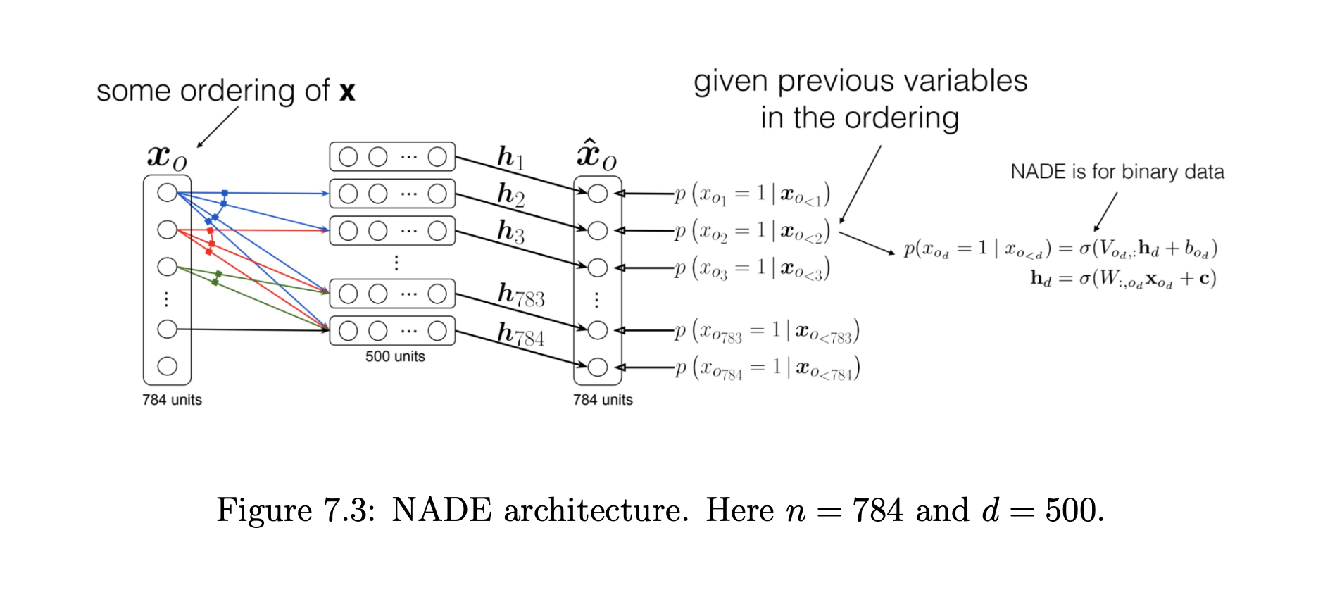
Neural Autoregressive Density Estimator (NADE)

Shares hidden-layer parameters across all conditionals to reduce complexity from $O(D^2)$ to $O(Dd)$, where $d$ is hidden size.
Model
1. Hidden activations \[ a_1 = c,\quad a_{i+1} = a_i + W_{:,\,i}\,x_i,\quad h_i = \sigma(a_i), \] where $W\in\mathbb{R}^{d\times D}$ and $c\in\mathbb{R}^d$ are shared.
2. Conditional probability \[ p(x_i=1 \mid x_{<i}) = \hat{x}_i = \sigma\bigl(b_i + V_{i,:}\,h_i\bigr), \] with $V\in\mathbb{R}^{D\times d}$ and $b\in\mathbb{R}^D$.
Properties
- Parameter count: $O(Dd)$ vs. $O(D^2)$ in FVSBN
- Computation: joint log-likelihood $\sum_i\log p(x_i\mid x_{<i})$ in $O(Dd)$ via one forward pass
Training
- Maximize average log-likelihood using teacher forcing (use ground-truth $x_{<i}$).
- Extensions: RNADE (real-valued inputs), DeepNADE (deep MLP), ConvNADE.
Inference
- Sequential sampling $x_1,\dots,x_D$, with optional random ordering for binary pixels.

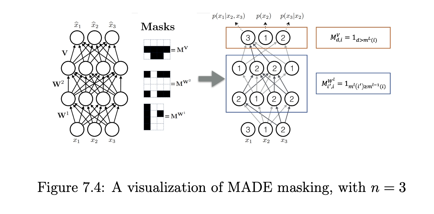
MADE (Masked Autoencoder for Distribution Estimation)

Adapts a feed-forward autoencoder to AR modeling by masking weights to enforce $x_i$ depends only on $x_{<i}$.
Masking
- Assign each unit an index $m\in\{1,\dots,D\}$.
- A weight from unit $u\to v$ is active only if $m(u)<m(v)$ (hidden layers) and $m(u)<i$ for output $x_i$.
Training & Generation
- Train by minimizing negative log-likelihood.
- Sequential sampling: $D$ forward passes, one per new $x_i$.
Ordering Robustness
- Randomizing masks/orders per epoch improves generalization.

AR Models for Images

PixelRNN

Uses RNNs (LSTM/GRU) over flattened pixels.
Dependency: Each pixel $x_i$ conditioned on RNN hidden state summarizing $x_{<i}$.
Ordering: Raster or diagonal scan; variants include Row LSTM, Diagonal BiLSTM.
Generation: $O(HW)$ sequential steps for $H\times W$ image.

PixelCNN

Uses masked convolutions to model $p(x_{r,c}\mid x_{\prec(r,c)})$.
Mask Types
1. Type A (first layer): blocks current pixel.
2. Type B (subsequent): allows self-connection but no future pixels.
Training
- Parallel over all pixels via masked convolution stacks.
Generation
- Sequential sampling $O(HW)$ steps.
Blind-Spot Issue
- Deep stacks can leave unconditioned “holes.” Gated PixelCNN or two-pass designs address this.

TCNs (Temporal Convolutional Networks) & WaveNet

TCN: 1D causal convolutions ensure $y_t$ depends only on $x_{\le t}$.
Dilated Convolutions
- Factor $d$: gaps between filter taps.
- Stack dilations $1,2,4,\dots$ for exponential receptive field growth.
WaveNet
- Masked, dilated convolutions on raw audio.
- Models long-range audio dependencies efficiently.

Variational RNNs (VRNNs) & C-VRNNs

VRNN
- Embeds a VAE at each timestep $t$.
- Prior: $p(z_t\mid h_t)=\mathcal{N}(\mu_{0,t},\mathrm{diag}(\sigma_{0,t}^2))$ where $(\mu_{0,t},\sigma_{0,t})=\phi_{\text{prior}}(h_t)$.
C-VRNN
- Conditions on external variables (e.g. control signals) alongside latent $z_t$.

Architecture Trade-offs for $p(x_i\mid x_{<i})$

RNNs
- Compress arbitrary history.
- Recency bias; vanishing distant signals.
CNNs (Masked/Dilated)
- Parallelizable; scalable receptive field.
- Fixed context; blind spots.
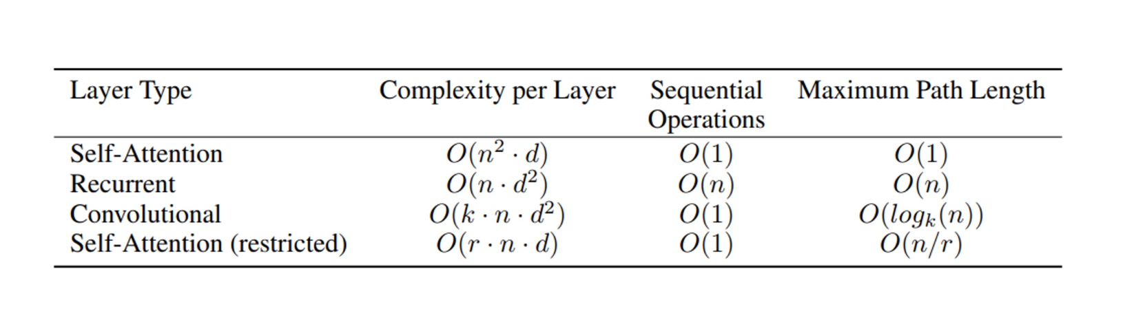
Transformers
- Masked self-attention to all $x_{<i}$.
- Highly parallel training.
- Quadratic $O(L^2)$ attention cost; need positional encoding.
Large Language Models (LLMs)
- Transformer-based AR on token sequences.
- Pretraining: next-token prediction.
- Fine-Tuning: supervised tasks (SFT).
- Tokenization: subword units (BPE, WordPiece).

AR for High-Resolution Images & Video

Challenge: Millions of pixels/voxels → $O(D)$ sequential steps infeasible.
Approach: Compress data into discrete latent sequences via VQ-VAE.

Vector-Quantized VAE (VQ-VAE)

Objective: Learn a discrete latent representation for high-dimensional data, enabling compact encoding and efficient autoregressive modeling.
Model Components:
- Encoder:
  - A convolutional neural network (CNN) mapping input
    $\mathbf{x}\in\mathbb{R}^{H\times W\times C}$ to continuous latents
    $\mathbf{z}_e(\mathbf{x})\in\mathbb{R}^{H'\times W'\times D}$.
  - Spatial down-sampling factor $s$: $H'=H/s,\;W'=W/s$ (e.g. $s=8$).
- Codebook:
  - A collection $\mathcal{E}=\{e_j\in\mathbb{R}^D\mid j=1,\dots,K\}$ of $K$ trainable embedding vectors.
- Quantization:
  - For each spatial cell $(p,q)$, take
    $z_e(\mathbf{x})_{p,q}\in\mathbb{R}^D$ and find nearest codebook index \[ k_{p,q} = \arg\min_{j\in\{1..K\}} \bigl\|z_e(\mathbf{x})_{p,q} - e_j\bigr\|_2^2. \]
  - Replace $z_e(\mathbf{x})_{p,q}$ with $e_{k_{p,q}}$, yielding discrete latents
    $\mathbf{z}_q(\mathbf{x})\in\mathbb{R}^{H'\times W'\times D}$.
- Decoder:
  - A CNN mapping $\mathbf{z}_q(\mathbf{x})$ back to a reconstruction
    $\hat{\mathbf{x}}\in\mathbb{R}^{H\times W\times C}$.
Loss Terms:
1. Reconstruction Loss: \[ L_{\mathrm{rec}} = \bigl\|\mathbf{x} - \hat{\mathbf{x}}\bigr\|_2^2. \]
2. Codebook Loss: (fix encoder, update codebook) \[ L_{\mathrm{cb}} = \sum_{p,q} \bigl\|\mathrm{sg}\bigl[z_e(\mathbf{x})_{p,q}\bigr] - e_{k_{p,q}}\bigr\|_2^2. \]
3. Commitment Loss: (fix codebook, update encoder) \[ L_{\mathrm{com}} = \beta \sum_{p,q} \bigl\|z_e(\mathbf{x})_{p,q} - \mathrm{sg}\bigl[e_{k_{p,q}}\bigr]\bigr\|_2^2, \] where $\beta$ (e.g. $0.25$) balances encoder commitment, and $\mathrm{sg}[\cdot]$ is stop‐gradient.
- Total Loss: \[ L_{\mathrm{VQ\text{-}VAE}} = L_{\mathrm{rec}} + L_{\mathrm{cb}} + L_{\mathrm{com}}. \]
Optimization Details:
- Straight-Through Estimator (STE):
  - Quantization is non-differentiable.
  - In backprop, pass gradients from $\mathbf{z}_q$ directly to $\mathbf{z}_e$ (i.e. treat quantization as identity).
- Codebook Updates via EMA (alternatively):
  - Maintain per‐embedding counts $N_j$ and sums $m_j$: \[ N_j \gets \gamma\,N_j + (1-\gamma)\sum_{p,q}\mathbf{1}[k_{p,q}=j], \] \[ m_j \gets \gamma\,m_j + (1-\gamma)\sum_{p,q:k_{p,q}=j} z_e(\mathbf{x})_{p,q}, \] then update \[ e_j \gets \frac{m_j}{N_j}, \] with decay $\gamma\approx0.99$.
Practical Considerations:
- Hyperparameters:
  - Codebook size $K$ (e.g. 512–1024), embedding dimension $D$ (e.g. 64–256).
  - Compression factor $s$ reduces sequence length from $HW$ to $H'W'$.
- Downstream Use:
  - After training, the discrete codes $\{k_{p,q}\}$ form a sequence of length $H'W'$.
  - An autoregressive model (e.g. Transformer) can be trained on these code sequences:
    \[p(k_{p,q}\mid k_{<p,q}).\]
- Intuition:
  - Each $e_j$ becomes a “prototype” latent vector.
  - The encoder emits a continuous vector, which is snapped to its nearest prototype, enforcing discreteness and preventing posterior collapse.

Generative Adversarial Networks (GANs)

Introduction

Origin and Context
- GANs were introduced by Goodfellow et al. in 2014.
- They became widely adopted and studied around 2016.
Implicit Generative Models
- GANs are implicit generative models: they learn to represent a data distribution $p_{data}(x)$ through a generative process, rather than by explicitly modeling the probability density function.
- The model does not require an explicit likelihood function.

Limitations of Likelihood-based Methods

Challenges in Likelihood Estimation
- Maximizing likelihood does not guarantee high-quality or representative samples.
  - A model may assign high likelihood to noisy or outlier regions, skewing the overall likelihood score, even if it fails to capture the main modes of the data.
Paradoxical Outcomes
- Models can achieve high likelihood scores while generating poor-quality samples.
- Conversely, models that generate visually realistic samples may have poor log-likelihood scores.
Memorization vs. Generalization
- Likelihood-based models may overfit and memorize the training data, achieving high likelihood on the training set but failing to generalize and generate novel samples.

GANs as Implicit Generative Models

Key Characteristics
- Likelihood-free: GANs do not require explicit definition or optimization of a likelihood function $p(x)$.
- Architectural Flexibility: The generator and discriminator can be implemented using various neural network architectures (e.g., MLP, CNN, RNN).
- Transformation: GANs map low-dimensional random noise vectors $z$ to high-dimensional structured data samples $G(z)$.
- Sample Quality: GANs often produce sharper and more realistic samples than Variational Autoencoders (VAEs), especially for images.
- Composability: GANs can be integrated with other generative models (e.g., VAEs, Normalizing Flows, Diffusion Models) to potentially improve sample quality or training stability.

Architecture Components

Generator Network ($G$)
- Input: Latent vector $z$ sampled from a prior distribution $p_z(z)$ (e.g., standard Gaussian $\mathcal{N}(0, I)$ or Uniform $U[-1, 1]$).
- Output: Synthetic data sample $x_{fake} = G(z)$, in the same space as the real data.
- Objective: Generate samples $G(z)$ that are indistinguishable from real data samples $x \sim p_{data}(x)$.
Discriminator Network ($D$)
- Input: Data sample $x$, which can be either a real sample ($x \sim p_{data}(x)$) or a fake sample ($x = G(z)$).
- Output: Scalar probability $D(x) \in [0, 1]$, representing the estimated probability that $x$ is a real sample from $p_{data}(x)$.
- Objective: Accurately classify inputs as real ($D(x) \to 1$) or fake ($D(G(z)) \to 0$).

Training Dynamics

Adversarial Framework
- The process is a zero-sum, two-player minimax game between $G$ and $D$.
  - $G$ tries to fool $D$ by generating increasingly realistic samples.
  - $D$ tries to improve its ability to distinguish real samples from fake ones generated by $G$.
- Training involves backpropagating gradients: $D$’s gradients guide its own learning, and also flow back through $D$ (when frozen) to train $G$.
Mathematical Formulation
- The core value function $V(G, D)$ defines the minimax objective: \[ \min_G \max_D V(G, D) = \mathbb{E}_{x \sim p_{data}(x)}[\log D(x)] + \mathbb{E}_{z \sim p_z(z)}[\log(1 - D(G(z)))] \]
Optimization
- $D$ is trained to maximize $V(G, D)$ (maximize classification accuracy).
- $G$ is trained to minimize $V(G, D)$ (minimize the log-probability of $D$ being correct about fake samples).
Theoretical Equilibrium (Nash Equilibrium)
- If $G$ and $D$ have sufficient capacity and training converges optimally:
  - The generator’s distribution $p_g$ matches the real data distribution $p_{data}$.
  - The discriminator outputs $D(x) = 1/2$ everywhere, unable to distinguish real from fake.
- Assumptions: This requires strong assumptions like infinite model capacity and the ability to find the Nash equilibrium, which are often not met in practice.

Practical Training Algorithm

Alternating Optimization
- Simultaneous gradient descent for minimax games is unstable, so training typically alternates:
  - Train Discriminator: Freeze $G$, update $D$ for one or more ($k$) steps by ascending its gradient: $\nabla_D V(G, D)$.
  - Train Generator: Freeze $D$, update $G$ for one step by descending its gradient: $\nabla_G V(G, D)$.
  - Repeat.
- Often $k > 1$ (e.g., $k=5$) to ensure $D$ remains relatively well-optimized.
Training Considerations
- Balance: Crucial to maintain balance between $G$ and $D$. If $D$ becomes too strong too quickly, gradients for $G$ can vanish. If $D$ is too weak, $G$ receives poor guidance.
- Computational Cost: Training is computationally intensive due to the need to train two networks and potentially perform multiple discriminator updates per generator update.

Proposition 1: Optimal Discriminator

For a fixed generator $G$, the optimal discriminator $D^*(x)$ that maximizes $V(G, D)$ is:

\[ D^*(x) = \frac{p_{data}(x)}{p_{data}(x) + p_g(x)} \]

where $p_g(x)$ is the probability density of the samples generated by $G$.
Derivation:
- The discriminator’s objective is: \[ \max_D \mathbb{E}_{x \sim p_{data}}[\log D(x)] + \mathbb{E}_{z \sim p_z}[\log(1 - D(G(z)))] \]
- By the law of the unconscious statistician, this can be rewritten as: \[ \max_D \int_x p_{data}(x) \log D(x) dx + \int_x p_g(x) \log(1 - D(x)) dx \]
- For each $x$, maximize $a \log y + b \log(1-y)$ with $a = p_{data}(x)$, $b = p_g(x)$, $y = D(x)$.
- The maximum is at $y^* = \frac{a}{a+b}$, so: \[ D^*(x) = \frac{p_{data}(x)}{p_{data}(x) + p_g(x)} \]

Proposition 2: GANs Minimize Jensen-Shannon Divergence

When $D$ is optimal ($D^*$), the training objective for $G$ corresponds to minimizing the Jensen-Shannon (JS) divergence between $p_{data}$ and $p_g$.
Kullback-Leibler (KL) Divergence: \[ D_{KL}(P || Q) = \int P(x) \log \frac{P(x)}{Q(x)} dx \]
Jensen-Shannon (JS) Divergence: \[ D_{JS}(P || Q) = \frac{1}{2} D_{KL}(P || M) + \frac{1}{2} D_{KL}(Q || M) \] where $M = \frac{1}{2}(P + Q)$. $0 \le D_{JS}(P || Q) \le \log 2$.
Proof Sketch:
- Substitute $D^*(x)$ into $V(G, D)$: \[ \begin{aligned} C(G) &= \max_D V(G, D) = V(G, D^*) \\ &= \mathbb{E}_{x \sim p_{data}}[\log D^*(x)] + \mathbb{E}_{x \sim p_g}[\log(1 - D^*(x))] \\ &= \mathbb{E}_{x \sim p_{data}}\left[\log \frac{p_{data}(x)}{p_{data}(x) + p_g(x)}\right] + \mathbb{E}_{x \sim p_g}\left[\log \frac{p_g(x)}{p_{data}(x) + p_g(x)}\right] \\ &= \int p_{data}(x) \log \frac{p_{data}(x)}{2 \cdot \frac{1}{2}(p_{data}(x) + p_g(x))} dx + \int p_g(x) \log \frac{p_g(x)}{2 \cdot \frac{1}{2}(p_{data}(x) + p_g(x))} dx \\ &= \int p_{data}(x) \left( \log \frac{p_{data}(x)}{m(x)} - \log 2 \right) dx + \int p_g(x) \left( \log \frac{p_g(x)}{m(x)} - \log 2 \right) dx \\ &= (D_{KL}(p_{data} || m) - \log 2) + (D_{KL}(p_g || m) - \log 2) \\ &= D_{KL}(p_{data} || m) + D_{KL}(p_g || m) - 2 \log 2 \\ &= 2 D_{JS}(p_{data}, p_g) - 2 \log 2 \end{aligned} \]
- Minimizing $C(G)$ with respect to $G$ is equivalent to minimizing $D_{JS}(p_{data}, p_g)$, as $-2 \log 2$ is a constant.
- The minimum value of $D_{JS}$ is $0$, achieved if and only if $p_{data} = p_g$.

Practical Training Algorithm (continued)

The theoretical analysis assumes $D$ can always reach its optimum $D^*$ for any $G$, but in practice, $D$ is only optimized for a finite number of steps ($k$), and this inner-loop optimization is computationally intensive and can lead to overfitting on finite datasets.
Alternating optimization (typically $k \in \{1, ..., 5\}$ steps for $D$ per $G$ update) is used to keep $D$ near optimal while allowing $G$ to change slowly.

Issues with Training

Vanishing Gradients
- Problem: When $D$ is very confident (outputs close to 0 or 1) and accurate, the gradient $\log(1 - D(G(z)))$ for $G$ can become very small (saturate), especially early in training when $G$ produces poor samples easily distinguishable by $D$. This stalls the learning of $G$.
- Solution (Non-Saturating Loss): Instead of minimizing $\mathbb{E}_{z \sim p_z(z)}[\log(1 - D(G(z)))]$, the generator maximizes $\mathbb{E}_{z \sim p_z(z)}[\log D(G(z))]$. This provides stronger gradients early in training. The generator’s objective becomes: \[ \mathcal{L}_G = - \mathbb{E}_{z \sim p_z(z)}[\log D(G(z))] \]
Mode Collapse
- Problem: The generator $G$ learns to produce only a limited variety of samples, collapsing many modes of the true data distribution $p_{data}$ into one or a few output modes. $G$ finds a few samples that can easily fool the current $D$, and stops exploring.
- Potential Causes: $G$ finds a local minimum in the adversarial game.
- Mitigation Strategies:
  - Architectural changes
  - Alternative loss functions (e.g., Wasserstein GAN, which uses the Wasserstein distance as a similarity measure between distributions, providing smoother gradients and better mode coverage)
  - Unrolled GANs: The generator is optimized with respect to the state of $D$ after the next $k$ steps, discouraging $G$ from exploiting local minima.
  - Mini-batch discrimination and gradient accumulation can also help.
Training Instability
- Problem: The adversarial training process involves finding a Nash equilibrium, which is inherently more unstable than standard minimization problems. Updates improving one player ($G$ or $D$) might worsen the objective for the other, leading to oscillations or divergence.
- Mitigation Strategies:
  - Careful hyperparameter tuning
  - Architectural choices (e.g., Spectral Normalization)
  - Gradient penalties (e.g., WGAN-GP adds a penalty term related to the norm of the discriminator’s gradient with respect to its input, often evaluated at points interpolated between real and fake samples: $\|\nabla_{\hat{x}} D(\hat{x})\|_2$).
    - Explanation: In WGAN-GP, the gradient penalty enforces the Lipschitz constraint by penalizing the squared deviation of the gradient norm from 1: \[ \lambda \mathbb{E}_{\hat{x}} \left( \|\nabla_{\hat{x}} D(\hat{x})\|_2 - 1 \right)^2 \] where $\hat{x}$ is sampled uniformly along straight lines between pairs of points from the real and generated data distributions.

StyleGANs

Overview
- StyleGANs are a family of GAN architectures known for generating high-resolution, high-fidelity images (e.g., 1024x1024 faces).
Key Innovations
- Progressive Growing (introduced in PGGAN, adopted by StyleGAN)
  - Training starts with low-resolution images (e.g., 4x4).
  - New layers are progressively added to both $G$ and $D$ to increase the resolution (e.g., 8x8, 16x16, …), fine-tuning the network at each stage. This stabilizes training for high resolutions.
- Style-Based Generator
  - Mapping Network: A separate network (e.g., an MLP) maps the initial latent code $z \sim p_z(z)$ to an intermediate latent space $W$. This disentangles the latent space. $w \in W$.
  - Adaptive Instance Normalization (AdaIN): The intermediate latent $w$ is transformed into style parameters (scale $\mathbf{y}_s$ and bias $\mathbf{y}_b$) which modulate the activations at each layer of the synthesis network. \[ \text{AdaIN}(x_i, w) = \mathbf{y}_{s,i} \frac{x_i - \mu(x_i)}{\sigma(x_i)} + \mathbf{y}_{b,i} \] where $x_i$ are the activations of the $i$-th feature map, $\mu(x_i)$ and $\sigma(x_i)$ are the mean and standard deviation, and $\mathbf{y}_{s,i}, \mathbf{y}_{b,i}$ are learned affine transformations applied to $w$.
  - Constant Input & Noise Injection: The synthesis network starts from a learned constant tensor instead of the latent code directly. Stochasticity (e.g., hair placement, freckles) is introduced by adding learned per-pixel noise at each layer, scaled by learned factors.
  - Hierarchical Control: Injecting $w$ (via AdaIN) at different layers controls different levels of attributes: early layers affect coarse features (pose, shape), while later layers affect finer details (color scheme, micro-textures).

Image-to-Image Translation

Task: Learn a mapping function to translate an image from a source domain A to a target domain B (e.g., segmentation maps to photos, sketches to photos, day to night).
Pix2Pix
- A conditional GAN (cGAN) approach where the generator is conditioned on the input image from domain A. $G: A \to B$.
- Requires Paired Data: Training needs datasets where each image $x_A$ has a corresponding ground truth image $x_B$.
- Loss Function: Combines a conditional GAN loss (discriminator $D$ tries to distinguish real pairs $(x_A, x_B)$ from fake pairs $(x_A, G(x_A))$) with a reconstruction loss, typically L1 loss: \[ \mathcal{L}_{L1}(G) = \mathbb{E}_{x_A, x_B}[||x_B - G(x_A)||_1] \] L1 loss is often preferred over L2 (MSE) as it encourages less blurring in the generated images.
- Architecture: Often uses a “U-Net” architecture for the generator and a “PatchGAN” discriminator (classifies patches of the image as real/fake).
CycleGAN
- Designed for Unpaired Data: Can learn translations when there is no direct one-to-one mapping between images in domain A and domain B (e.g., translating photos of horses to zebras, or photographs to Monet paintings).
- Architecture: Uses two generators ($G_{A \to B}$ and $G_{B \to A}$) and two discriminators ($D_A$ and $D_B$).
  - $G_{A \to B}$: Translates A to B. $D_B$: Distinguishes real B images from generated $\hat{x}_B = G_{A \to B}(x_A)$.
  - $G_{B \to A}$: Translates B to A. $D_A$: Distinguishes real A images from generated $\hat{x}_A = G_{B \to A}(x_B)$.
- Cycle Consistency Loss: Ensures that translating an image from A to B and back to A should recover the original image (and vice-versa). \[ \mathcal{L}_{cyc}(G_{A \to B}, G_{B \to A}) = \mathbb{E}_{x_A}[||G_{B \to A}(G_{A \to B}(x_A)) - x_A||_1] + \mathbb{E}_{x_B}[||G_{A \to B}(G_{B \to A}(x_B)) - x_B||_1] \]
- Total Loss: Sum of the adversarial losses for both mappings and the cycle consistency loss. \[ \mathcal{L}_{total} = \mathcal{L}_{GAN}(G_{A \to B}, D_B) + \mathcal{L}_{GAN}(G_{B \to A}, D_A) + \lambda \mathcal{L}_{cyc}(G_{A \to B}, G_{B \to A}) \] where $\lambda$ is a hyperparameter controlling the cycle consistency term.

Other Applications & Extensions

Video-to-Video Translation (Vid2Vid)
- Extends image translation to video, requiring temporal consistency across generated frames.
3D GANs
- Generate 3D shapes or scenes, often represented as voxel grids, point clouds, or implicit neural representations.

Normalizing Flows (NFs)

Core Concepts

Definition
- Normalizing Flows (NFs) are generative models that represent a complex data distribution $p(x)$ by transforming a simple base distribution $p_Z(z)$ (e.g., Gaussian) through an invertible and differentiable function $f: \mathcal{Z} \to \mathcal{X}$, where $x = f(z)$.
Tractable Likelihood
- NFs allow exact likelihood computation using the change of variables formula. Given $z = f^{-1}(x)$: \[ p_X(x) = p_Z(z) \left| \det \left( \frac{\partial z}{\partial x} \right) \right| = p_Z(f^{-1}(x)) \left| \det J_{f^{-1}}(x) \right| \]
- Alternatively, by the inverse function theorem ($J_f(z) = (J_{f^{-1}}(x))^{-1}$): \[ p_X(x) = p_Z(z) \left| \det J_f(z) \right|^{-1} \]
Requirements for Transformation $f$
- Invertible: $f^{-1}$ must exist.
- Differentiable: Both $f$ and $f^{-1}$ must be differentiable (i.e., $f$ is a diffeomorphism).
- Efficient Jacobian Determinant: The determinant of the Jacobian matrix ($\det J_f$ or $\det J_{f^{-1}}$) must be computationally efficient (ideally $O(D)$ or $O(D^2)$ for $D$ dimensions, not $O(D^3)$ as in the general case). This is often achieved by using triangular or structured Jacobians.
- Dimensionality Preservation: The input and output dimensions must match, i.e., $\dim(x) = \dim(z)$.
Composition
- Complex transformations are constructed by composing multiple simpler invertible layers: $f = f_L \circ \dots \circ f_1$.
- The overall log-determinant is the sum of the log-determinants of each layer: \[ \log p_X(x) = \log p_Z(z) + \sum_{i=1}^L \log \left| \det J_{f_i^{-1}}(x_i) \right| \] where $x_i$ is the input to layer $f_i^{-1}$.
Inference vs. Sampling
- Likelihood Evaluation (Inference): Compute $z = f^{-1}(x)$ and evaluate $p_X(x)$ using the above formula.
- Sampling: Sample $z \sim p_Z(z)$ and compute $x = f(z)$.

Key Building Block: Coupling Layers

Concept
- Partition input dimensions $x$ into two parts, $x = (x_a, x_b)$. Transform one part ($x_a$) based on the other ($x_b$), while leaving $x_b$ unchanged: \[ y_a = h(x_a; \theta(x_b)) \] \[ y_b = x_b \]
- $h$ must be invertible with respect to $x_a$.
- $\theta(x_b)$ can be arbitrarily complex and does not have to be invertible.
Example: Affine Coupling Layer
- $h(x_a; s, t) = x_a \odot s + t$, where $(s, t) = \theta(x_b)$.
Forward Pass
- $y_a = h(x_a, \theta(x_b))$
- $y_b = x_b$
Backward Pass
- $x_a = h^{-1}(y_a, \theta(y_b))$
- $x_b = y_b$
Jacobian Matrix
- The Jacobian is block lower triangular: \[ J = \frac{\partial y}{\partial x} = \begin{pmatrix} \frac{\partial y_a}{\partial x_a} & \frac{\partial y_a}{\partial x_b} \\ 0 & I \end{pmatrix} \]
Determinant
- The determinant is efficient to compute: \[ \det(J) = \det \left( \frac{\partial y_a}{\partial x_a} \right) = \det \left( \frac{\partial h(x_a; \theta(x_b))}{\partial x_a} \right) \]
- For affine coupling layers, $\frac{\partial y_a}{\partial x_a} = \mathrm{diag}(s)$, so $\det(J) = \prod_i s_i$.
Conditioning
- To make the flow conditional on external information $c$, modify the parameter network: $(s, t) = \theta(x_b, c)$. The Jacobian structure remains unchanged.
Transformation Composition
- The overall transformation is a composition of all the transformations, and the determinants multiply (log-determinants sum).
- Since one part of the input is untransformed in each layer, the next layer should transform this part, or at each step, a different mask of features should be used.
Training
- Maximize the exact log-likelihood of i.i.d. samples, so the density is explicitly defined.
Inference
- To sample, draw $z$ from the base distribution and pass it through the transformations.
- To compute the sample probability, use invertibility to transform $x$ back to $z$ and measure its probability.
Continuous Normalizing Flows
- Allow modeling of arbitrarily complex distributions by parameterizing the transformation as a continuous-time ODE.

Architectural Patterns (e.g., RealNVP, GLOW)

General Patterns
- The main differences in architectures are in the choice of $h$ and how variables are split.
NICE Model
- An early flow-based model using an additive coupling layer and splitting variables as $x_{1:d}$ and $x_{d+1:D}$, where $D$ is the input dimension.
Multi-Scale Architecture
- Employs sequences of blocks operating at different spatial resolutions.

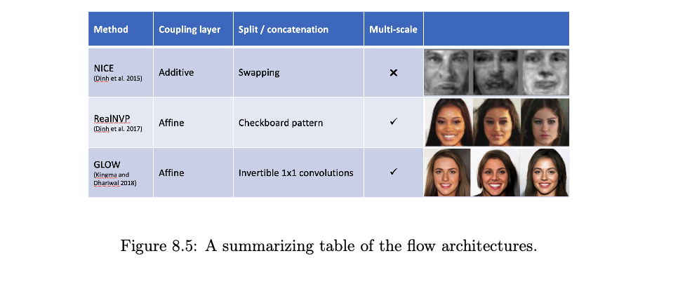
RealNVP

Utilizes a combination of spatial checkerboard pattern, channel-wise masking, and affine mapping.
The split operation partitions the input data using a spatial checkerboard pattern, followed by a squeeze operation and channel-wise masking.
The squeeze operation reduces the spatial dimensions while increasing the number of channels. For an input tensor of size $W \times H \times C$, the squeeze operation transforms it to $W/2 \times H/2 \times 4C$ by dividing the input into $2 \times 2$ subsquares and assigning elements to different channels in a clockwise rotation.
The coupling layer uses an affine mapping: \[ y_A = x_A \odot \exp(s(x_B)) + t(x_B) \] \[ y_B = x_B \] where $s$ and $t$ can be arbitrarily complex (e.g., neural networks), $\odot$ denotes element-wise product, and $y_A$, $y_B$ are the resulting partitions.
The Jacobian is triangular, so its log-determinant is efficiently computed as $\sum s(x_B)$.

GLOW

Introduced invertible $1 \times 1$ convolutions and affine coupling layers.
Each flow step consists of:
1. Activation Normalization (ActNorm)
  - Normalizes each input channel by learning a per-channel scale $s$ and bias $b$.
  - Forward: $y_{i,j} = s \odot x_{i,j} + b$
  - Reverse: $x_{i,j} = (y_{i,j} - b)/s$
  - Log-determinant: $H \cdot W \cdot \sum \log(|s|)$
2. Invertible $1 \times 1$ Convolution
  - Generalizes permutation in the channel dimension.
  - The convolution weight matrix $W \in \mathbb{R}^{C \times C}$ is initialized as a random rotation matrix with $\det(W) = 1$.
  - To compute the determinant efficiently, $W$ is parameterized using LU decomposition: \[ W = P \cdot L \cdot (U + \mathrm{diag}(s)) \] where $P$ is a fixed permutation matrix, $L$ is lower triangular with ones on the diagonal, $U$ is upper triangular, and $s$ is a vector.
  - Log-determinant: $\sum \log |s|$
3. (Conditional) Coupling Layer
  - As in RealNVP, but with channel-wise splitting.
  - $x_A, x_B = \mathrm{split}(x)$
  - $(\log s, t) = \mathrm{NN}(x_B)$
  - $s = \exp(\log s)$
  - $y_A = s \odot x_A + t$
  - $y_B = x_B$
  - $y = \mathrm{concat}(y_A, y_B)$
Split Operation
- After a block, a fraction of dimensions (channels) can be split off and passed directly to the latent space $z$, reducing computational cost in subsequent layers.

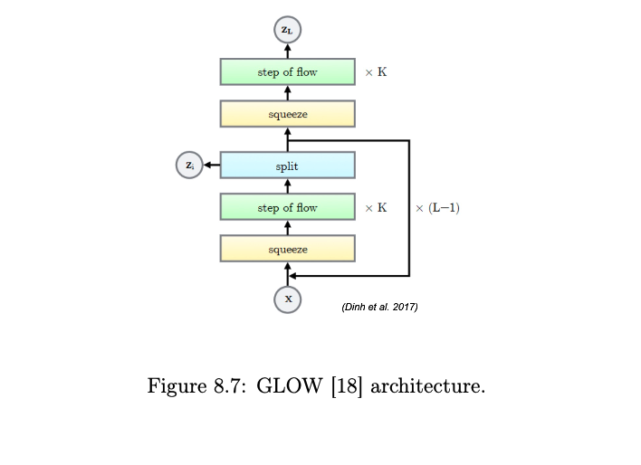
Notable NF Models

GLOW
- Introduced invertible $1 \times 1$ convolutions, achieving high-quality image generation for NFs at the time.
SRFlow
- Uses a conditional NF for super-resolution, modeling $p(x_{HR} | x_{LR})$.
StyleFlow
- Enables controlled, disentangled editing of images by applying a conditional NF to the latent space ($\mathcal{W}$ or $\mathcal{W}+$) of a pre-trained StyleGAN generator.
- Learns $w' = f(w; a_{target})$ where $w$ is the original StyleGAN latent, $a_{target}$ are desired attributes, and $w'$ is the edited latent.
- Training uses triplets $\{w, G(w), A(G(w))\}$, where $G$ is the StyleGAN generator and $A$ is an attribute predictor.
- The “forward” pass $w \to w'$ performs the edit. The “reverse” pass $w = f^{-1}(w'; a_{target})$ is also possible.

Conditional and Multimodal Flows

Conditional NFs
- Model $p(x|c)$ by making transformations dependent on conditioning variable $c$. Used in SRFlow, StyleFlow, etc.
C-Flows (Conditional Flows for Cross-Domain Generation)
- Link multiple data modalities (e.g., images $x_1$, point clouds $x_2$) through a shared latent space $z$.
- Learn flows $f_1: \mathcal{X}_1 \to \mathcal{Z}$ and $f_2: \mathcal{X}_2 \to \mathcal{Z}$.
- Allows generating data in one modality conditioned on another, e.g., generate $x_2$ from $x_1$ by computing $z = f_1^{-1}(x_1)$ and then sampling $x_2 = f_2(z)$.
- Training can be joint or conditional.

Limitations

Dimensionality Preservation
- Input and output dimensions must match, which can be computationally demanding for high-dimensional data, although techniques like splitting and multi-scale architectures mitigate this.
Sample Quality
- While offering tractable likelihoods, NFs sometimes lag behind Generative Adversarial Networks (GANs) and Diffusion Models in terms of photorealism for complex image generation tasks.
Topology
- Basic NFs cannot change the topology of the space; they are diffeomorphisms. [May not be a practical limitation for many tasks].

Applications in Computer Vision

Super-Resolution
- Learns a distribution of high-resolution variants.
Disentanglement
- Enables disentangled representation learning.
Multimodal Modeling
- Models joint or conditional distributions over multiple modalities.
3D Shape Modeling
- Models complex 3D shapes.
3D Pose Estimation
- Models distributions over 3D poses.
Regularization
- Provides explicit log-likelihoods for regularization in other models.

Diffusion Models

Definition: Diffusion models are explicit generative models that gradually add noise to data and learn to reverse this process to generate new samples.
Core Processes:
- Forward Process: Systematically adds Gaussian noise to the original data over $T$ steps.
- Reverse Process: Learns to denoise step-by-step, generating new samples from noise.
Training Objective: The model is trained to predict the noise added at each step, not the denoised data directly.
Advantages Over Other Generative Approaches
- Normalizing Flows: Require invertibility and tractable Jacobians; diffusion models do not have this constraint.
- Variational Autoencoders (VAEs) and Autoregressive Models: VAEs and autoregressive models often produce lower-quality samples compared to diffusion models.
- Generative Adversarial Networks (GANs): GANs are difficult to train and prone to mode collapse; diffusion models offer more stable training and higher sample diversity.
- Hybridization: Diffusion models can be combined with GANs to enhance realism while maintaining stability.
Training Methodology
- Self-supervised Paradigm: The process of adding controlled noise acts as a natural supervision signal.
- Noise Scheduling:
  - Progressive Approach: Start with minimal noise and gradually increase it.
  - Schedulers: Linear and cosine schedules are common. Linear schedules can cause the image to become pure noise too quickly, making learning difficult in later steps.
- Computational Characteristics:
  - Generation requires multiple passes (one per denoising step), similar to autoregressive models.
Architecture
- Model Core: U-Net architecture is used, shared across all timesteps.
- Time Representation: The timestep is encoded (e.g., sinusoidal encoding) and input to the model.
- Conditioning Approaches:
  - Classifier Guidance:
    - Adjusts noise prediction using a classifier trained on noisy images.
    - Can be added post-training.
    - Limitations:
      - Requires a classifier trained for all noise levels.
      - May introduce additional noise.
      - Limited to predefined class sets.
  - Direct Conditioning:
    - Embeds class labels or text directly into the model.
    - More flexible and effective than classifier guidance.
    - Must be implemented during training.
  - Classifier-Free Guidance (CFG):
    - Conditioning signal (e.g., text embedding) is applied only a fraction (e.g., 80%) of the time during training.
    - Model learns both conditional and unconditional denoising.
    - Increases output diversity.
    - Typically uses a CLIP embedding (Contrastive Language-Image Pre-training).
    - A hyperparameter controls the guidance strength.
    - Drawback: Slower generation, as both conditional and unconditional predictions are needed at each step.
Efficiency Enhancements
- Latent Diffusion Models (LDMs):
  - Diffusion is performed in a compressed latent space, not pixel space.
  - Pipeline: Encoder $\rightarrow$ Diffusion in latent space $\rightarrow$ Decoder.
  - Focuses on semantic content, not pixel-level details.
  - Key Idea: A Variational Autoencoder (VAE) is pre-trained to map images to a low-dimensional latent space. The VAE is frozen during diffusion model training.
  - Benefits: Operating in latent space reduces dimensionality and computational cost, improving efficiency.
  - Applications: Powers state-of-the-art systems such as Stable Diffusion, DALL-E, and Sora. [Verification Needed: Sora’s exact architecture.]
Advanced Applications
- Image-Conditioned Generation:
  - Conditioning on images (e.g., sketches, structures).
  - ControlNet:
    - Feature modulation approach.
    - Base diffusion model is frozen.
    - Parallel adaptation block with “zero convolution” layers (1x1 conv, zero-initialized).
    - Zero initialization ensures gradual adaptation without disrupting the base model.
  - Photo Relighting: Modifies lighting while preserving content.
Mathematical Foundation
- Forward Diffusion Process
  - Modeled as a Markov process with $T$ steps (typically $T \approx 1000$).
  - At each step $t$, Gaussian noise is added: \[ q(x_t|x_{t-1}) = \mathcal{N}(x_t; \sqrt{1-\beta_t}x_{t-1}, \beta_t\mathbf{I}) \] where $\beta_t$ is the noise schedule parameter.
  - Define $\alpha_t = 1 - \beta_t$ and $\bar{\alpha}_t = \prod_{i=1}^{t} \alpha_i$.
  - Using the reparameterization trick, sample $x_t$ given $x_0$: \[ x_t = \sqrt{\bar{\alpha}_t}x_0 + \sqrt{1-\bar{\alpha}_t}\epsilon, \quad \epsilon \sim \mathcal{N}(0, \mathbf{I}) \] \[ q(x_t | x_0) = \mathcal{N}(\sqrt{\bar{\alpha}_t} x_0, (1-\bar{\alpha}_t) \mathbf{I}) \]
- Reverse Diffusion Process
  - The goal is to learn $p_\theta(x_{t-1}|x_t)$ to approximate the true reverse process.
  - By Bayes’ rule: \[ q(x_{t-1}|x_t,x_0) = \frac{q(x_t|x_{t-1},x_0)q(x_{t-1}|x_0)}{q(x_t|x_0)} \]
  - All terms are Gaussian, so $q(x_{t-1}|x_t,x_0)$ is Gaussian with:
    - Mean: \[ \tilde{\mu}_t(x_t,x_0) = \frac{\sqrt{\alpha_t}(1-\bar{\alpha}_{t-1})}{1-\bar{\alpha}_t}x_t + \frac{\sqrt{\bar{\alpha}_{t-1}}\beta_t}{1-\bar{\alpha}_t}x_0 \]
    - Variance: \[ \tilde{\beta}_t = \frac{1-\bar{\alpha}_{t-1}}{1-\bar{\alpha}_t}\beta_t \]
Training Objective
- Model $p_\theta(x_{t-1}|x_t)$ as a Gaussian with:
  - Fixed variance $\tilde{\beta}_t$ (from the forward process).
  - Learned mean $\mu_\theta(x_t,t)$ (predicted by a neural network).
- ELBO Derivation:
  - Maximize the log-likelihood $\log p_\theta(x_0)$ via the Evidence Lower Bound (ELBO): \[ \log p_\theta(x_0) \geq \mathbb{E}_{q(x_{1:T}|x_0)}\left[\log\frac{p_\theta(x_{0:T})}{q(x_{1:T}|x_0)}\right] = \mathcal{L}_\text{ELBO} \]
  - Expand the joint distributions: \[ p_\theta(x_{0:T}) = p(x_T) \prod_{t=1}^{T} p_\theta(x_{t-1}|x_t) \]
  - Rewrite the forward process using Bayes’ rule:
    - Start with the chain rule factorization: \[ q(x_{1:T}|x_0) = q(x_T|x_0) \cdot q(x_{T-1}|x_T, x_0) \cdot q(x_{T-2}|x_{T-1}, x_T, x_0) \cdots q(x_1|x_2, \ldots, x_T, x_0) \]
    - Apply the Markov property: given $x_{t+1}$ and $x_0$, $x_t$ is independent of future states: \[ q(x_t|x_{t+1}, x_{t+2}, \ldots, x_T, x_0) = q(x_t|x_{t+1}, x_0) \]
    - This gives us the key factorization: \[ q(x_{1:T}|x_0) = q(x_T|x_0) \prod_{t=1}^{T-1} q(x_t|x_{t+1}, x_0) \]
  - Substitute and rearrange: \[ \mathcal{L}_\text{ELBO} = \mathbb{E}_q\left[\log\frac{p(x_T) \prod_{t=1}^{T} p_\theta(x_{t-1}|x_t)}{q(x_T|x_0) \prod_{t=1}^{T-1} q(x_t|x_{t+1}, x_0)}\right] \] \[ = \mathbb{E}_q\left[\log\frac{p(x_T)}{q(x_T|x_0)} + \log p_\theta(x_0|x_1) + \sum_{t=1}^{T-1}\log\frac{p_\theta(x_t|x_{t+1})}{q(x_t|x_{t+1}, x_0)}\right] \]
  - Decomposed into three terms: \[ \mathcal{L}_\text{ELBO} = \mathcal{L}_T + \mathcal{L}_0 + \mathcal{L}_{1:T-1} \]
    - Prior Matching Term ($\mathcal{L}_T$): \[ \mathcal{L}_T = \mathbb{E}_q\left[\log \frac{p(x_T)}{q(x_T|x_0)}\right] = -D_\text{KL}(q(x_T|x_0) \| p(x_T)) \]
      - For large $T$, $q(x_T|x_0) \approx \mathcal{N}(0,\mathbf{I})$ and $p(x_T) = \mathcal{N}(0,\mathbf{I})$, so this term is negligible.
    - Reconstruction Term ($\mathcal{L}_0$): \[ \mathcal{L}_0 = \mathbb{E}_{q(x_1|x_0)}[\log p_\theta(x_0|x_1)] \]
      - Measures how well the final denoising step reconstructs the original data.
    - Denoising Matching Terms ($\mathcal{L}_{1:T-1}$): \[ \mathcal{L}_{1:T-1} = \sum_{t=1}^{T-1}\mathbb{E}_q\left[\log \frac{p_\theta(x_t|x_{t+1})}{q(x_t|x_{t+1}, x_0)}\right] = -\sum_{t=1}^{T-1}D_\text{KL}(q(x_t|x_{t+1}, x_0) \| p_\theta(x_t|x_{t+1})) \]
      - Measures how well the learned reverse process matches the true denoising transitions.
- Simplified Training Objective:
  - If $p_\theta(x_{t-1}|x_t)$ is Gaussian with the same variance as $q(x_{t-1}|x_t,x_0)$, the KL divergence in $\mathcal{L}_{1:T-1}$ reduces to the squared error between means.
  - The training loss becomes: \[ \mathcal{L} = \mathbb{E}_{t,x_0,\epsilon} \left[ \|\epsilon - \epsilon_\theta(x_t, t)\|^2 \right] \] \[ \left\|\epsilon-\hat{\epsilon}_{\Theta}\left(\sqrt{\overline{\alpha_t}} \mathbf{x}_{0}+\sqrt{1-\overline{\alpha_t}} \epsilon, t\right)\right\|^2 \]
  - $\epsilon_\theta(x_t, t)$ is the network’s prediction of the noise component.
- Training Algorithm
  
  \[ \begin{aligned} &\text{Algorithm: Diffusion Model Training} \\ &\text{while not converged do} \\ &\quad \mathbf{x}_0 \sim q(\mathbf{x}_0) \\ &\quad t \sim \mathcal{U}(\{1, \ldots, T\}) \\ &\quad \epsilon \sim \mathcal{N}(\mathbf{0}, \mathbf{I}) \\ &\quad \mathbf{x}_t = \sqrt{\bar{\alpha}_t} \mathbf{x}_0 + \sqrt{1-\bar{\alpha}_t} \epsilon \\ &\quad \text{Take gradient step on } \nabla_{\Theta}\left\|\epsilon-\epsilon_{\Theta}\left(\mathbf{x}_t, t\right)\right\|^2 \\ &\text{end while} \end{aligned} \]
- Sampling Algorithm
  - Start from $x_T \sim \mathcal{N}(0, \mathbf{I})$.
  - For $t = T$ down to $1$:
    - Predict noise: $\hat{\epsilon} = \epsilon_\theta(x_t, t)$.
    - Compute mean: \[ \mu_\theta(x_t, t) = \frac{1}{\sqrt{\alpha_t}}\left(x_t - \frac{\beta_t}{\sqrt{1-\bar{\alpha}_t}}\hat{\epsilon}\right) \]
    - If $t > 1$, sample: \[ x_{t-1} = \mu_\theta(x_t, t) + \sqrt{\tilde{\beta}_t}z, \quad z \sim \mathcal{N}(0, \mathbf{I}) \]
    - Else, set $x_0 = \mu_\theta(x_1, 1)$.
Additional Resources
- What are diffusion models?
- Tutorial on vision diffusion models
- Understanding diffusion models

Foundation Models

General Concept
- Train a large network to perform well on a wide range of tasks, often with minimal or no task-specific fine-tuning.
Historical Progression
- First Generation: ELMo, BERT, ERNIE
  - Model is pre-trained, then a task-specific decoder is added.
- Second Generation: GPT-3
  - Generalized model, fine-tuned for specific tasks.
- Third Generation: ChatGPT, DeepSeek
  - Zero-shot and few-shot learning; models are instruction-tuned and can generalize to new tasks with little or no additional training.
Vision Foundation Models
- Tokenization: Images are split into patches, which are linearly projected and fed into a transformer.
- Vision Transformer (ViT, 2020):
  - Linear projection of flattened patches.
  - Uses a transformer encoder.
  - Includes a learnable class embedding token (CLS token) to represent the whole image.
- Masked Autoencoder (MAE) Pretraining:
  - Randomly masks patches and trains the model to reconstruct them.
  - Enables joint prediction, depth estimation, and image inpainting. [Verification Needed: “joint prediction” is ambiguous.]
- SAM (Segment Anything Model, Meta):
  - Promptable segmentation model.
  - Requires large-scale labeled data, often refined with human-in-the-loop annotation.
- CLIP:
  - Shared embedding space for image and text.
  - Trained with contrastive learning on image-text pairs.
  - Enables dot product similarity for retrieval and zero-shot classification.
- DINO:
  - Self-distillation without labels.
  - Student matches the output of a teacher (an EMA of the student).
  - Teacher sees the whole image; student sees a crop.
  - Teacher is fixed and updated only via the student for stability.
  - Enables extraction of general features with zero supervision.
Multimodal Models
- 4M (EPFL) - Massively Multimodal Masked Modeling:
  - Any-to-any model: can handle image-to-text, normals, depth, 3D, etc.
  - All modalities are tokenized, randomly masked, and the model is trained to predict all modalities.
  - Requires knowledge of labels for each modality.
  - Pseudo-labeling can be used, leveraging state-of-the-art models for each task.
- DreamBooth:
  - Customized text-to-image generation.
  - Fine-tunes a diffusion model on a few examples of a specific subject, associating it with a unique token.
- Zero1to3:
  - Fine-tunes a diffusion model with 3D data.
  - From a single image, generates multiple views (novel view synthesis).

Parametric Human Body Models

Goals

Develop methods for perceiving and understanding human motion.
Learn techniques for generating and mimicking human motion.
Key research areas:
- Body Representation: Mathematical and structural modeling of the human body.
- Feature Representation Learning: Extraction of meaningful features from data (e.g., images, sensors) to inform body models.

Human Perception Insights

Humans can infer motion from sparse visual cues (e.g., a few moving points representing joints).
Human visual perception involves significant cognitive interpretation beyond raw sensory input.

Challenges in Human Pose and Shape Estimation

Depth Ambiguity: Inferring 3D structure from 2D projections is inherently ambiguous.
Self-Occlusion: Body parts can obscure other parts from view.
Low Contrast: Difficulty distinguishing the subject from the background or due to clothing.
Viewpoint Variations: Changes in camera angle or subject rotation.
Aspect Ratio and Scale Variations: Humans appear at different sizes and proportions in images.
Inter-Person Variability: High diversity in human body shapes.

Early Models

Pictorial Structures:
- Represent the body as a collection of parts (nodes) connected by spring-like potentials (edges), forming a graphical model.
- Primarily used for 2D pose estimation.

Key Questions in the Field

How can human body structure be effectively represented for computational analysis?
What features are most relevant for accurately estimating human pose and shape, and how can they be learned?

Feature Representation Learning for 2D Pose Estimation

Direct Regression Methods

Example: DeepPose
- Utilizes Convolutional Neural Networks (CNNs) for end-to-end feature extraction from images.
- Assumes global image features (from a person crop or the entire image) contain sufficient information for direct regression of pose parameters.
- Outputs 2D keypoint coordinates (e.g., $(x, y)$ pairs) directly.
- Often incorporates iterative refinement, where initial predictions are fed back into the network for improved accuracy.

Heatmap Regression Methods

Example: Convolutional Pose Machines (CPM) (2016)
- Predicts a probability distribution (heatmap) for each keypoint’s location over the image plane.
- More robust than direct coordinate regression, especially for handling occlusions and ambiguities.
- Typically, one heatmap is predicted per keypoint type (e.g., left elbow, right knee), which are then combined in a final stage to form the full pose.
- Architecture and Process:
  - Input: Single RGB image.
  - Multi-stage CNN architecture.
  - The initial stage produces a coarse estimate of keypoint heatmaps.
  - Subsequent stages refine these heatmaps by leveraging both image features and the belief maps (heatmaps) from previous stages. This iterative process allows the network to implicitly learn spatial context and part relationships.
  - Each stage is typically supervised during training, guiding the network towards progressively more accurate heatmap predictions.
  - Iterative refinement significantly improves keypoint localization accuracy.

Combining Body Modeling with Deep Representation Learning

Use predicted keypoint heatmaps from deep networks.
Refine these predictions jointly by incorporating explicit body model constraints (e.g., kinematic constraints, limb length ratios).
Employ spatial-temporal inference by considering sequences of images/frames to ensure temporal consistency and smoothness of motion.

OpenPose: Realtime Multi-Person 2D Keypoint Estimation (2017)

Approach: Bottom-up. Detects all potential keypoints in an image and then groups them into individual skeletons.
Does not require prior person detection or cropping, enabling detection in crowded scenes.
Architecture:
- Branch 1 (Keypoint Localization): Multi-stage CNN, similar to CPM, predicts heatmaps for all body parts.
- Branch 2 (Part Association): Predicts Part Affinity Fields (PAFs).
  - PAFs are 2D vector fields encoding the position and orientation of limbs (connections between pairs of keypoints).
  - Used to associate detected keypoints belonging to the same person, assembling individual skeletons from the pool of detected parts.
Addresses the challenge of associating parts to individuals in multi-person scenarios.

ViTPose: Vision Transformer for Top-Down Pose Estimation (2022)

Approach: Top-down.
Relies on an external person detector to first identify and crop individual instances in the image.
Pose estimation is then performed independently on each cropped image patch.
Simplifies the pose estimation task for each instance.
Overall performance depends on the accuracy of the initial person detector.
Requires processing multiple cropped images if multiple people are present, potentially increasing computational load compared to bottom-up methods for crowded scenes.

General Notes on 2D Pose Estimation

Parameterization: 2D pose is straightforward to parameterize, typically as a set of 2D coordinates for predefined anatomical keypoints.
Datasets: Large-scale 2D datasets with human annotations (e.g., COCO, MPII Human Pose) are crucial for training deep learning models.
Limitations:
- Acquiring 3D annotations is significantly more challenging and expensive than 2D.
- Simple 2D keypoint representations do not capture the full complexity of the human body, such as its 3D shape, volume, and surface characteristics.
- There is a strong desire for richer representations that include 3D body shape and can model articulation in 3D space.

3D Human Body Models

Statistical Shape Modeling - Basel Face Model (BFM) (1999)

Description:
- A statistical 3D Morphable Model (3DMM) for human faces.
- Represents 3D face shapes (and often textures/albedo) as a linear combination of example faces from a database.
- Acts as a generative model, capable of producing novel 3D face geometries and appearances.
Construction:
- Built from a dataset of registered 3D scans of faces, requiring dense correspondence.
- Dense Correspondence: Establishes a one-to-one mapping of vertices between a template mesh and all input scans, ensuring that vertices at the same index across different shapes correspond to the same semantic facial feature (e.g., tip of the nose).
- Bootstrapping Problem: Dense correspondence is needed to build the model, but a model can help establish dense correspondence. This is often addressed using iterative alignment and model refinement techniques.
Modeling:
- Principal Component Analysis (PCA) is used to learn a low-dimensional latent space for shape (and texture) from the registered scans.
- A new face shape $X$ (as a vector of vertex coordinates) can be synthesized as: \[ X = \bar{S} + Uc \] where:
  - $\bar{S}$ is the mean face shape vector,
  - $U$ is a matrix whose columns are the principal components (eigenvectors or “basis shapes”),
  - $c$ is a vector of shape coefficients (weights for each principal component). $$
- This linear model allows for continuous variation and generation of new, plausible face shapes by manipulating the coefficients $c$.
Fitting to an Image:
- Typically involves initializing a template mesh with an approximate pose and scale over a detected face in an image.
- An optimization procedure adjusts the shape coefficients $c$ (and potentially pose, illumination, and expression parameters) to best match the input image features (e.g., landmarks, edges, photometric appearance).
- Output: A 3D mesh representing the fitted face.

SMPL - Skinned Multi-Person Linear Model

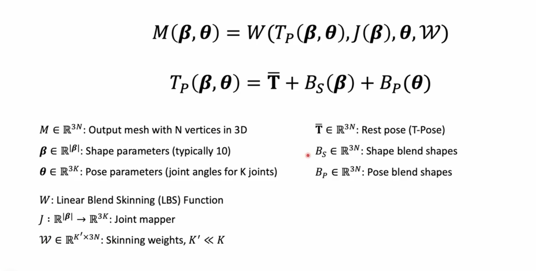
Description:
- A parametric, statistical model of the human body that outputs a 3D mesh and corresponding joint locations.
- Inputs: A vector of shape parameters ($\beta$) and a vector of pose parameters ($\theta$).
Core Components:
- Template Mesh ($\bar{T}$): A base 3D mesh with a fixed topology (standard SMPL has 6890 vertices), typically in a canonical pose (e.g., T-pose or A-pose). $\bar{T}$ often represents the mean shape.
- Shape Blend Shapes ($B_S(\beta; S)$):
  - Vertex offsets added to the template mesh to represent variations in body shape due to identity.
  - Defined as a linear combination: \[ B_S(\beta; S) = \sum_{k=1}^{|\beta|} \beta_k S_k \] where:
    - $S_k \in \mathbb{R}^{3N}$ are orthonormal basis shapes (e.g., learned via PCA from a dataset of registered 3D scans), $N$ is the number of vertices,
    - $\beta_k$ are scalar shape coefficients.
  - The shaped mesh in its rest pose (before posing) is $V_{shape} = \bar{T} + B_S(\beta; S)$.
- Joint Locations ($J(\beta; \mathcal{R})$):
  - The 3D locations of $K$ predefined joints (e.g., 23 in the basic SMPL model, plus a root) are regressed from the vertices of the shaped mesh in its rest pose: \[ J(\beta; \mathcal{R}) = \mathcal{R}(V_{shape}) \] where $\mathcal{R}$ is a learned regressor (e.g., a linear regression matrix).
- Pose ($\theta$):
  - Represents body articulation as a set of 3D rotations for each of the $K$ joints relative to its parent in a kinematic tree structure.
  - SMPL uses an axis-angle representation for joint rotations, so $\theta_k \in \mathbb{R}^3$ for each joint $k$.
  - The full pose vector $\theta \in \mathbb{R}^{(K+1) \times 3}$ includes the global orientation of the body and the relative rotations of $K$ joints.
- Pose Blend Shapes ($B_P(\theta; P)$):
  - Corrective vertex offsets added to the shaped rest mesh to mitigate artifacts from standard Linear Blend Skinning (LBS), such as joint collapse or the “candy-wrapper” effect during extreme rotations.
  - Dependent on the input pose $\theta$. The formulation is: \[ B_P(\theta; P) = \sum_{m=1}^{9K} (R_m(\theta) - R_m(\theta^*)) P_m \] where:
    - $R(\theta): \mathbb{R}^{(K+1) \times 3} \rightarrow \mathbb{R}^{9K}$ maps the axis-angle pose vector $\theta$ to a vector of concatenated $3 \times 3$ rotation matrix elements for $K$ joints (each $3 \times 3$ matrix has 9 elements),
    - $R_m(\theta)$ is the $m$-th element of this vectorized rotation matrix representation,
    - $\theta^*$ represents the rest pose (e.g., T-pose),
    - $P_m \in \mathbb{R}^{3N}$ are learned pose-corrective basis displacement vectors, $P = [P_1, ..., P_{9K}] \in \mathbb{R}^{3N \times 9K}$ is the matrix of all pose blend shape bases.
    - Subtracting $R_m(\theta^*)$ ensures that $B_P(\theta^*; P) = 0$, so pose blend shapes have no effect in the rest pose.
- Linear Blend Skinning (LBS):
  - Standard algorithm in computer graphics to deform mesh vertices according to the rotations of the articulated skeleton.
  - The mesh to be deformed by LBS is the template mesh modified by both shape and pose blend shapes: \[ V_{posed\_rest} = \bar{T} + B_S(\beta; S) + B_P(\theta; P) \]
  - Each vertex $v_i$ of $V_{posed\_rest}$ is transformed by a weighted sum of the transformations $G_j(\theta, J(\beta; \mathcal{R}))$ of its influencing joints: \[ v'_i = \sum_{j=0}^{K} w_{i,j} G_j(\theta, J(\beta; \mathcal{R})) v_i \] where:
    - $v'_i$ is the final transformed vertex,
    - $w_{i,j}$ are the skinning weights, defining the influence of joint $j$ on vertex $v_i$ (learned parameters in SMPL),
    - $G_j(\theta, J(\beta; \mathcal{R}))$ is the global rigid transformation (rotation and translation) of joint $j$ in world space, derived from the pose parameters $\theta$ and the joint locations $J(\beta; \mathcal{R})$ through forward kinematics.
- Final Model Output Function:
  - The complete SMPL model $M(\beta, \theta; \bar{T}, S, P, \mathcal{R}, W)$ generates the final posed 3D mesh vertices: \[ M(\beta, \theta) = \text{LBS}(\bar{T} + B_S(\beta; S) + B_P(\theta; P), J(\beta; \mathcal{R}), \theta, W) \]
  - The parameters to the right of the semicolon ($\bar{T}, S, P, \mathcal{R}, W$) are learned model parameters, while $\beta$ and $\theta$ are user inputs.

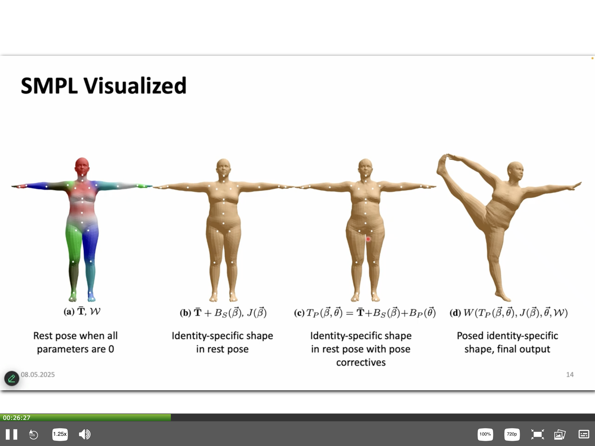
Learning SMPL:
- The model parameters (template $\bar{T}$, shape bases $S$, pose bases $P$, joint regressor $\mathcal{R}$, and skinning weights $W$) are learned by optimizing them to fit a large dataset of 3D body scans of different individuals in various poses.
Challenges in Registration for Learning SMPL:
- Aligning high-resolution, often noisy, and incomplete scan data to the SMPL template mesh topology.
- Handling complex poses, self-contact, and smooth, featureless areas on the body surface during registration.
Optimization during Learning:
- Typically involves minimizing an objective function that includes data terms (e.g., Euclidean distance between registered scan vertices and corresponding model vertices) and regularization terms (e.g., to ensure smooth shapes, prevent interpenetration, enforce plausible joint limits).
- Co-registration techniques might be employed, where model parameters and scan-to-model correspondences are optimized simultaneously or iteratively.

Human Mesh Recovery (HMR) (2018)

Methodology:
- Deep learning-based approach to directly regress SMPL parameters (pose $\theta$, shape $\beta$) and camera parameters from a single input image.
- The regressed parameters are then fed into the SMPL model to generate a 3D mesh.
- Often employs an adversarial training setup:
  - A discriminator network is trained to distinguish between SMPL parameters regressed from images and those obtained from “real” 3D scan data (or mocap data), encouraging the regressor to produce more realistic and plausible body configurations.

SMPLify / SMPLify-X (SMPLify: 2016; SMPLify-X: 2019)

Methodology:
- Optimization-based approach to fit the SMPL model (or its extensions like SMPL-X, which includes hands and face articulation) to 2D evidence extracted from an image.
Process:
- Initialize SMPL parameters (e.g., to a mean pose/shape, or from an initial estimate by a regression network).
- Iteratively optimize the pose $\theta$ and shape $\beta$ parameters (and potentially camera parameters, global translation) to minimize an objective function.
- The objective function typically includes:
  - Data Term: Penalizes the discrepancy between the 2D projection of 3D SMPL joints and detected 2D keypoints in the image. Silhouettes or other cues can also be used.
  - Shape Prior: Encourages plausible body shapes, often by penalizing $\beta$ coefficients that deviate significantly from a learned distribution (e.g., a Gaussian prior, $\|\beta\|^2$).
  - Pose Prior: Penalizes unnatural or impossible poses. This can be implemented using priors learned from motion capture (mocap) data, such as joint angle limits or models for interpenetration avoidance.
- Unlike HMR, SMPLify does not directly regress parameters from image features via a deep network; instead, it relies on pre-detected 2D (or sometimes 3D) landmarks and performs an iterative optimization.

Fitting SMPL to IMU Measurements

Methodology:
- Utilizes data from Inertial Measurement Units (IMUs), which typically consist of accelerometers and gyroscopes, attached to various body segments.
- IMU data provides orientation (and derivatives like angular velocity, linear acceleration) for these segments.
- This sensor data can be used to estimate joint orientations ($\theta$) and subsequently fit the SMPL model, often in real-time.
- Electromagnetic sensors can also provide positional and orientational data for similar fitting procedures.
Challenges:
- Sensor Drift: IMUs, particularly gyroscopes, are prone to integration drift over time, leading to orientation errors.
- Magnetic Disturbances: Electromagnetic sensors can be affected by metallic objects or magnetic fields in the environment.
- Sparsity: Mapping data from a sparse set of sensors to a full-body pose.
- Calibration: Accurate sensor-to-segment calibration (aligning sensor axes with body segment coordinate systems) is crucial.

Modeling Clothing on Parametric Bodies

Limitations of SMPL: The base SMPL model represents a minimally-clothed or naked body. Clothing is not explicitly part of its learned parameters or fixed topology.
Approaches for Modeling Clothing on SMPL-like Bodies:
- Displacement Maps: Learning vertex displacements from the base body surface to represent the geometry of relatively static clothing.
- Implicit Representations:
  - Using neural implicit functions, such as Signed Distance Functions (SDFs) or occupancy fields, conditioned on body pose, shape, and potentially clothing type/style parameters to model the clothed surface.
  - Animated Neural Implicit Surfaces: A promising research direction for modeling dynamic clothed humans, where the implicit surface deforms according to body motion and learned or simulated clothing dynamics.
- Explicit Clothed Avatars:
  - Learning separate geometric models for individual garments.
  - Combining these garment models with the body model, often involving physics-based simulation for realistic cloth behavior or data-driven deformation techniques.
Challenges:
- Clothing introduces significant geometric complexity and dynamic behavior (wrinkles, folds, material properties) not captured by SMPL’s fixed topology or LBS.
- Modeling the vast diversity of clothing types, their interactions with the body, and material properties remains a complex task.

Egocentric Vision

Egocentric vision is the study of visual data captured from a first-person perspective, typically using wearable cameras. This perspective is inherently dynamic, uncurated, and embodied, producing long-form video that reflects the agent’s goals, interactions, and attention.

Research Tasks

Key research tasks in egocentric vision include:

Localization
3D scene understanding
Anticipation (e.g., predicting future actions or object interactions)
Action recognition
Gaze understanding and prediction
Social behavior understanding
Full body pose estimation
Hand and hand-object interaction analysis
Person identification
Privacy (addressing challenges and developing solutions)
Summarization of long-form egocentric video
Visual question answering (VQA) in egocentric contexts
Robotic applications (using egocentric perception for robot control and interaction)

Hand and Hand-Object Interaction

Understanding hand use and hand-object interactions is central to egocentric vision.

Understanding Human Hands in Contact at Internet Scale (Shan et al., 2020):
- Goal: Extract hand state and contact information from internet videos.
- Dataset: 100DOH, with 131 days of footage and 100,000 annotated hand-contact frames across 12 categories and 27,300 videos. Annotations include hand and object bounding boxes, left/right hand labels, and contact states (none, self, person, portable, non-portable object).
- Technical Approach: Uses Faster-RCNN to predict, for each hand, the bounding box, left/right label, and contact state.
- Results: Achieved 90% hand detection accuracy; demonstrated automated 3D hand mesh reconstruction and grasp pose prediction for uncontacted objects.
DexYCB Dataset:
- Focuses on object manipulation and interaction, relevant for both human and robotic contexts.
- Provides data for:
  - 2D object and keypoint detection
  - 6D object pose estimation (3D translation and 3D rotation)
  - 3D hand pose estimation
- Offers higher quantity and quality than alternatives like HO-3D, with manual annotations and improved robustness for multiple views.
HaMeR (Pavlakos et al., 2024):
- State-of-the-art model for 3D hand mesh reconstruction from monocular images.
- Based on a Vision Transformer (ViT)-like architecture, predicting parameters of the MANO hand model.
- End-to-end: takes monocular images and left/right hand information as input, outputs a 3D hand mesh.
- Robust tracking, with failures mainly in extreme poses.
- Introduces the HInt dataset with annotated 2D keypoints from multiple sources.

Action Recognition and Anticipation

Predicting future actions and intentions from egocentric video is a major challenge.

Challenge: Modeling human intentions requires understanding past actions and context from long-form egocentric videos.
Summarize the Past to Predict the Future (Pasca et al., CVPR 2024):
- Goal: Improve short-term object interaction anticipation using natural language descriptions of past context.
- Task: Predict the object (noun), action (verb), and time to contact (TTC) for future interactions.
- Previous Approaches: Ego4D Faster R-CNN + SlowFast baseline, AFF-tention (Mur-Labadia et al., ECCV 2024).
- Method:
  - Language Context Extraction: Applies object detection and image captioning to past frames. A VQA model with prompts (e.g., “What does the image describe?”, “What is the person in this image doing?”) extracts verbose descriptions. Part-of-speech tagging, lemmatization, and majority voting aggregate verbs and nouns. Filtering removes out-of-domain verb-noun pairs. CLIP identifies salient objects for context extraction without extra training.
  - TransFusion Model: Multimodal fusion model that combines language context and visual features to predict future action (verb, noun) and TTC.
- Results: Outperforms vision-only baselines on the Ego4D Short Term Object Interaction Anticipation Dataset (v1 and v2), especially for both frequent and infrequent noun and verb classes.
PALM: Predicting Actions through Language Models (Kim et al., ECCV 2024):
- Idea: Leverage procedural knowledge in large language models (LLMs) for action anticipation.
- Approach:
  1. Prompt Generation: Image captioning and action recognition models process egocentric frames to generate a visual context description and a sequence of past actions (verb, noun pairs).
  2. Action Anticipation: An LLM is prompted with the visual context, past actions, and a template instruction to predict a sequence of future actions (verb, noun pairs). In-context learning with examples is used. Maximal Marginal Relevance (MMR) is used for exemplar selection.
- Qualitative Comparison: Achieves lower edit distance between predicted and ground truth future action sequences compared to a SlowFast baseline, indicating better sequence prediction.

Gaze Understanding and Prediction

Estimating the camera wearer’s gaze is a fundamental egocentric vision task.

Egocentric Gaze Estimation (Lai et al., BMVC 2022):
- Problem: Estimate the visual attention of the camera wearer from egocentric videos.
- Previous Challenge: Eye trackers required calibration, increasing cost and complexity.
- Approach: Introduces the first transformer-based model for egocentric gaze estimation, incorporating global context via a global-local correlation module. Argues that local token correlations are insufficient; global context is necessary.
- Task: Predict a probability map indicating gaze location.
Leveraging Driver Field-of-View for Multimodal Ego-Trajectory Prediction (Akbiyik et al., ICLR 2025):
- Goal: Improve ego-trajectory prediction (predicting the future path of the camera wearer) by incorporating driver field-of-view (gaze) data alongside scene videos.
- Dataset: Gaze-assisted Ego Motion (GEM) Dataset.
- Framework:
  - Inputs: past trajectory $M_{1:T}$, scene videos $S_{1:T}$, and FOV data ($V_{F_{1:T}}$ for visual features, $G_{F_{1:T}}$ for gaze data) over 8 seconds.
  - Video encoders $E_S$ process scene videos.
  - A cross-modal transformer integrates visual features and FOV data.
  - Modal embeddings are stacked and processed by a multimodal encoder $E_M$ with self-attention.
  - A time-series transformer predicts the future trajectory $M'_{T+1:T_{pred}}$ (6 seconds) and future FOV $F_{T+1:T_{pred}}$.
  - Note: No gradient flows from trajectory prediction to the multimodal encoder during training, only from predicted future FOV.
  - Losses: visual loss $\mathcal{L}_V$ for future FOV and trajectory loss $\mathcal{L}_T$ for future trajectory.
- Path Complexity Index (PCI): Defined as \[ PCI(\mathcal{T}_{\text{target}} \| \mathcal{T}_{\text{input}}) = \mathcal{T}_{\text{target}}(t) - \mathcal{T}_{\text{simple}}(t) \] Used to measure the complexity or curvature of a predicted path relative to a simple baseline path.
  [Verification Needed: The formula needs clarification on how $\mathcal{T}_{\text{simple}}(t)$ is derived.]
- Results: Incorporating gaze data improves ego-trajectory prediction performance.

3D Scene Understanding

Interpreting the 3D environment from egocentric video is challenging due to camera motion and a narrow field of view.

Challenge: Camera motion and limited field of view make it difficult to understand spatial layout and object relationships. 3D interpretation helps contextualize actions and compensates for camera movement.
Epic Fields: Marrying 3D Geometry and Video Understanding (Tschernezki et al., NeurIPS 2023):
- Concept: Proposes the Lift, Match, and Keep (LMK) approach for dynamic 3D scene understanding from egocentric video.
- LMK Approach:
  - Lift: Convert 2D observations from video frames to 3D world coordinates.
  - Match: Connect observations of the same object over time using appearance and estimated 3D location.
  - Keep: Maintain object tracks even when temporarily out of view.
- Dataset: Evaluated on a dataset derived from EPIC-KITCHENS, with 100 long videos (25 hours) across 45 kitchens and 2,939 objects.
- Performance: Achieved object tracking accuracy of 64% after 1 minute, 48% after 5 minutes, and 37% after 10 minutes, outperforming baselines.
EgoGaussian: Dynamic Scene Understanding from Egocentric Video with 3D Gaussian Splatting (Zhang et al., 3DV 2025):
- Explores the use of 3D Gaussian Splatting for representing and understanding dynamic scenes from egocentric video.

Robotic Applications

Egocentric vision is highly relevant for robot perception and control, especially for dexterous manipulation.

Kitten Carousel (Heid & Hein, 1963): Classic experiment showing the importance of self-motion and visual feedback for perceptual development. Kittens with control over their movement developed normal depth perception, while passive kittens did not, highlighting the value of embodied vision.
Visual Encoder for Dexterous Manipulation:
- Idea: Learn visual features for dexterous manipulation directly from egocentric videos.
- Motivation: Robot policy learning typically involves direct environment interaction; egocentric videos provide rich human manipulation data.
- Applications: Robotic control, interaction prediction, motion synthesis.
MAPLE: Encoding Dexterous Robotic Manipulation Priors Learned From Egocentric Videos (Heid et al., CVPR 2025):
- Goal: Learn manipulation priors from large-scale egocentric video pretraining to improve dexterous robotic manipulation.
- Approach:
  - Large-scale Egocentric Pretraining: Train a visual encoder (e.g., ViT-B/16) on egocentric videos to learn hand pose and contact point representations.
  - Label Extraction Pipeline: [Details needed; likely involves hand tracking, 3D hand pose estimation, and contact point identification.]
  - MAPLE Model: Takes prediction frames from egocentric video and outputs prior-infused features. Uses a Transformer Decoder to predict manipulation outputs, including contact points (2D coordinates) and a hand pose token (quantized hand pose index).
  - Dexterous Simulation Environments: Simulated environments train policies using prior-infused features.
  - Real-World Application: Learned priors are transferred to real robots for dexterous tasks.
- DiT - Policy: Diffusion transformer-based policy that takes prior-infused features as input and predicts action chunks (e.g., end effector pose in $SE(3)$, hand joints in $\mathbb{R}^{21}$).
- Evaluation: Evaluated in simulation and real-world on tasks like “Grab the plush animal,” “Place the pan,” and “Paint the canvas.” Showed improved success rates over baselines; failure cases included not grasping or releasing objects.
GEM: Egocentric World Foundation Model (Hassan et al., CVPR 2025):
- Goal: Develop a generalizable ego-vision multimodal world model for fine-grained ego-motion, object dynamics, and scene composition control.
- Comparison with Cosmos (Nvidia’s World Foundation Model):
  - Data: GEM uses 4K hours vs. 20M hours for Cosmos.
  - Compute: 0.5K GPUs for 3 days vs. 10K GPUs for 90 days.
  - Scale: 2B parameters vs. 14B.
  - Inference Time: 3 minutes vs. 10 minutes.
  - Extra Capabilities: Multimodal outputs (RGB and depth), fine-grained motion control, agent/object insertion, open-source dataset/code/models.
- Architecture: [Details needed; likely diffusion-based generative modeling for future frames and states.]
- Summary: GEM is more efficient and versatile than larger models like Cosmos, excelling in multimodal outputs and fine-grained control.

Summary

Egocentric vision is a critical and rapidly evolving area in computer vision.
Major challenges remain in understanding intentions, dynamic scenes, and privacy.
Large, diverse datasets (e.g., EPIC-KITCHENS, Ego4D) are driving progress.
There are many opportunities for impactful research in this field.

Implicit Surfaces, Neural Radiance Fields (NeRFs), and 3D Gaussian Splatting

This lecture extends 2D model generation concepts to 3D, focusing on representations, rendering, and learning methods for 3D scenes.

3D Representations

Voxels
- Discretize 3D space into a regular grid of volumetric pixels (voxels).
- Memory complexity is cubic: $O(N^3)$ for an $N \times N \times N$ grid.
- Resolution is limited by grid size.
Point Primitives / Volumetric Primitives
- Represent geometry as a collection of points (point cloud) or simple volumetric shapes (e.g., spheres).
- Do not explicitly encode connectivity or topology.
- Easily acquired with depth sensors (e.g., LiDAR).
Meshes
- Composed of vertices (points), edges (connections), and faces (typically triangles).
- Limited by the number of vertices; low resolution can cause self-intersections.
- Some methods require class-specific templates, but general mesh learning is also common.
- Remain popular due to compatibility with standard rendering pipelines.

Implicit Surfaces

Explicit vs. Implicit Shape Representation
- Explicit (mesh-like): Defined by discrete vertices and faces; representation is discontinuous.
- Implicit: Defined by a function $f(x, y) = 0$ (e.g., a circle: $x^2 + y^2 - r^2 = 0$); representation is continuous.
  - To compute $\frac{dy}{dx}$ for $F(x, y) = 0$ (e.g., $x^2 + y^2 - 1 = 0$): \[ \begin{aligned} \frac{d}{dx}[x^2 + y^2] &= \frac{d}{dx}[1] \\ 2x + 2y \frac{dy}{dx} &= 0 \\ \frac{dy}{dx} &= -\frac{x}{y} \end{aligned} \]
  - More generally, for $F(x, y) = 0$: \[ \frac{dy}{dx} = -\frac{\partial F / \partial x}{\partial F / \partial y} \] (assuming $\partial F / \partial y \neq 0$).
Level Sets
- Represent the surface as the zero level set of a continuous function $f: \mathbb{R}^3 \to \mathbb{R}$: \[ S = \{ \mathbf{x} \in \mathbb{R}^3 \mid f(\mathbf{x}) = 0 \} \]
- $f$ can be approximated by a neural network $f_\theta(\mathbf{x})$.
Signed Distance Functions (SDFs)
- $f(\mathbf{x})$ gives the signed distance from $\mathbf{x}$ to the surface; sign indicates inside/outside.
- Storing SDFs on a grid leads to $O(N^3)$ memory and limited resolution.
Neural Implicit Representations (e.g., Occupancy Networks, DeepSDF)
- Neural network predicts occupancy probability or SDF value for any $\mathbf{x} \in \mathbb{R}^3$.
Can be conditioned on class labels or images.
Advantages:
- Low memory (just network weights).
- Continuous, theoretically infinite resolution.
- Can represent arbitrary topologies.

Neural Fields

Neural fields generalize neural implicit representations to predict not only geometry but also color, lighting, and other properties.
Surface Normals from SDFs
- Surface normal at $\mathbf{x}$: $\mathbf{n}(\mathbf{x}) = \nabla f(\mathbf{x}) / \| \nabla f(\mathbf{x}) \|$.
- Computed efficiently via auto-differentiation.
- Used for regularization (e.g., Eikonal term).

Training Neural Implicit Surfaces

Supervision Levels (from easiest to hardest for geometry learning):
1. Watertight Meshes
  - Sample points and query occupancy or SDF.
  - Train with cross-entropy (occupancy) or regression (SDF).
2. Point Clouds
  - Supervise so that $f_\theta(\mathbf{x}) \approx 0$ for observed points.
3. Images
  - Requires differentiable rendering to compare rendered and real images.
Visualizing Implicit Surfaces
- Evaluate $f_\theta(\mathbf{x})$ on a grid and extract a mesh (e.g., Marching Cubes).
Overfitting for Representation
- Networks can be trained to overfit a single shape/class, compressing it into the weights.
- For implicit surfaces, this means accurate 3D reconstruction, not novel view synthesis.
Eikonal Regularization
- Enforces $\| \nabla f(\mathbf{x}) \| = 1$ for SDFs.
- Encourages smooth, well-behaved level sets.
- Loss: \[ L = \sum_{\mathbf{x}} |f_\theta(\mathbf{x})| + \lambda \sum_{\mathbf{x}} (\| \nabla f_\theta(\mathbf{x}) \| - 1)^2 \]
- Alternatively, an L1 penalty: \[ L = \sum_{\mathbf{x}} |f_\theta(\mathbf{x})| + \lambda \sum_{\mathbf{x}} |\| \nabla f_\theta(\mathbf{x}) \| - 1| \]

Differentiable Rendering for Neural Fields

Goal: Learn $f_\theta$ (geometry) and $t_\theta$ (texture) from 2D images by rendering and comparing to ground truth.
Rendering Pipeline:
1. For each pixel $u$, cast a ray $\mathbf{r}(d) = \mathbf{r}_0 + \mathbf{w}d$.
2. Find intersection $\hat{\mathbf{p}}$ where $f_\theta(\hat{\mathbf{p}}) = \tau$ (e.g., $\tau = 0$).
  - Use root-finding (e.g., Secant method) between samples with opposite signs.
3. Query $t_\theta(\hat{\mathbf{p}})$ for color.
4. Assign color to pixel $u$.
Forward Pass:
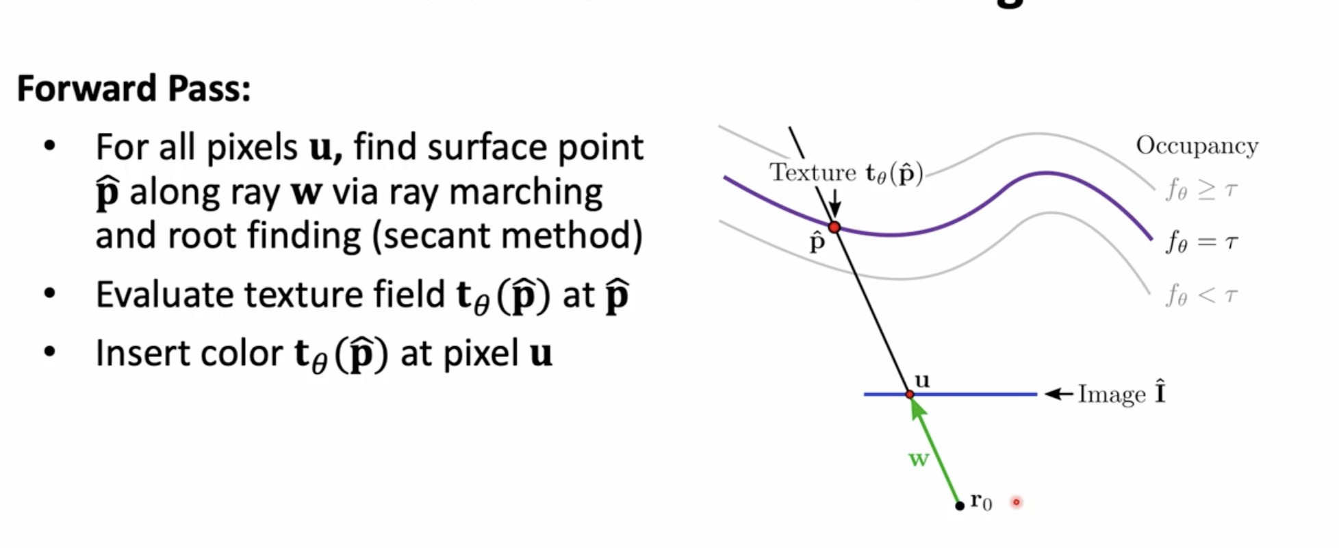
Backward Pass:
- For loss $L(I, \hat{I}) = \sum_u \| \hat{I}_u - I_u \|_1$.
- Where $\hat{I}_u = t_\theta(\hat{\mathbf{p}})$ is the rendered color at pixel $u$, where both $t_\theta$ and $\hat{\mathbf{p}}$ depend on $\theta$. \[ \frac{\partial \hat{I}_u}{\partial \theta} = \frac{\partial t_\theta(\hat{\mathbf{p}})}{\partial \theta} + \nabla_{\hat{\mathbf{p}}} t_\theta(\hat{\mathbf{p}}) \cdot \frac{\partial \hat{\mathbf{p}}}{\partial \theta} \]
- Implicit differentiation for $\frac{\partial \hat{\mathbf{p}}}{\partial \theta}$: \[ f_\theta(\hat{\mathbf{p}}) = \tau \implies \frac{\partial f_\theta(\hat{\mathbf{p}})}{\partial \theta} + \nabla_{\hat{\mathbf{p}}} f_\theta(\hat{\mathbf{p}}) \cdot \frac{\partial \hat{\mathbf{p}}}{\partial \theta} = 0 \] \[ \frac{\partial \hat{\mathbf{p}}}{\partial \theta} = -\frac{\frac{\partial f_\theta(\hat{\mathbf{p}})}{\partial \theta}}{\nabla_{\hat{\mathbf{p}}} f_\theta(\hat{\mathbf{p}}) \cdot \mathbf{w}} \mathbf{w} \]

Neural Radiance Fields (NeRFs)

Motivation: Model complex scenes with thin structures, transparency, and view-dependent effects.
Task: Given images with known camera poses, learn a volumetric scene representation for novel view synthesis.
Network Architecture:
- Input: 3D point $\mathbf{x}$ and viewing direction $\mathbf{d}$.
- Output: Color $\mathbf{c}$ and density $\sigma$.
- Structure:
  1. $\mathbf{x}$ (after positional encoding) passes through several fully connected layers.
  2. Outputs $\sigma$ and a feature vector.
  3. $\mathbf{d}$ (after positional encoding) is concatenated with the feature vector.
  4. Final layers output view-dependent color $\mathbf{c}$.
- Density $\sigma$ depends only on $\mathbf{x}$; color $\mathbf{c}$ depends on both $\mathbf{x}$ and $\mathbf{d}$.
Positional Encoding:
- MLPs are biased toward low-frequency functions.
- Encode each input coordinate $p$ as: \[ \gamma(p) = (\sin(2^0 \pi p), \cos(2^0 \pi p), \ldots, \sin(2^{L-1} \pi p), \cos(2^{L-1} \pi p)) \]
- Typically $L=10$ for $\mathbf{x}$, $L=4$ for $\mathbf{d}$.
Volume Rendering Process:
- For each pixel, cast a ray $\mathbf{r}(t) = \mathbf{o} + t\mathbf{d}$.
- Sample $N$ points along the ray.
- For each sample $i$ at $t_i$:
  - Query MLP: $(\mathbf{c}_i, \sigma_i) = \text{MLP}(\mathbf{r}(t_i), \mathbf{d})$.
  - Compute $\delta_i = t_{i+1} - t_i$.
  - Compute opacity: $\alpha_i = 1 - \exp(-\sigma_i \delta_i)$.
  - Compute transmittance: $T_i = \prod_{j=1}^{i-1} (1 - \alpha_j)$, with $T_1 = 1$.
- Color Integration: \[ \hat{C}(\mathbf{r}) = \sum_{i=1}^{N} T_i \alpha_i \mathbf{c}_i \]
  - $N$: Number of samples along the ray.
  - $\mathbf{c}_i, \sigma_i$: Color and density from MLP at sample $i$.
  - $\delta_i$: Distance between samples.
  - $\alpha_i$: Opacity for interval $i$.
  - $T_i$: Transmittance up to sample $i$.
Hierarchical Volume Sampling (HVS):
- Use a coarse network to sample uniformly, then a fine network to sample more densely where $T_i \alpha_i$ is high.
Training & Characteristics:
- Volumetric, models transparency and thin structures.
- Geometry can be noisy compared to explicit surface methods.
- Requires many calibrated images.
- Rendering is slow due to many MLP queries.
- Original NeRF is for static scenes.
Animating NeRFs / Dynamic Scenes
- Use a canonical space (e.g., T-pose) and learn a deformation field to map to observed poses.
- Find correspondences between observed and canonical space (may require a separate network).
- If multiple correspondences, select or aggregate (e.g., max confidence) [Verification Needed].
- Example: Vid2Avatar.
Alternative Parametrizations
- Use explicit primitives (e.g., voxels, cubes) with local NeRFs.
- Point-based primitives (e.g., spheres, ellipsoids) with neural features can be optimized and rendered efficiently.
- Ellipsoids better capture thin structures than spheres.

3D Gaussian Splatting (Kerbl et al., 2023)

Overview: Represents a scene as a set of 3D Gaussians, each with learnable parameters, and renders by projecting and compositing them.
Process:
1. Initialization:
  - Start from a sparse point cloud (e.g., from Structure-from-Motion).
  - Initialize one Gaussian per point.
2. Optimization Loop:
  - Project 3D Gaussians to 2D using camera parameters.
  - Render using a differentiable rasterizer (often tile-based).
  - Compute loss (e.g., L1, D-SSIM) between rendered and ground truth images.
  - Backpropagate to update Gaussian parameters.
3. Adaptive Density Control:
  - Prune Gaussians with low opacity or excessive size.
  - Densify by cloning/splitting in under-reconstructed regions.
Gaussian Parameters:
- 3D mean $\mathbf{\mu} \in \mathbb{R}^3$.
- 3x3 covariance $\mathbf{\Sigma}$ (parameterized by scale and quaternion for rotation).
- Color $\mathbf{c}$ (often as Spherical Harmonics coefficients).
- Opacity $o$ (scalar, passed through sigmoid).
Rendering:
- For each pixel:
  1. Project relevant 3D Gaussians to 2D.
  2. Sort by depth (front-to-back).
  3. For each Gaussian $i$:
    - Compute effective opacity at pixel: \[ \alpha_i' = o_i \cdot \exp\left(-\frac{1}{2} (\mathbf{p} - \mathbf{\mu}_i')^T (\mathbf{\Sigma}_i')^{-1} (\mathbf{p} - \mathbf{\mu}_i')\right) \]
      - $o_i$: Learned opacity.
      - $\mathbf{p}$: 2D pixel coordinate.
      - $\mathbf{\mu}_i'$: Projected 2D mean.
      - $\mathbf{\Sigma}_i'$: Projected 2D covariance.
    - Evaluate color $\mathbf{k}_i$ (from SH coefficients).
  4. Color Blending: \[ C = \sum_{i=1}^{N_g} \mathbf{k}_i \alpha_i' \prod_{j=1}^{i-1} (1 - \alpha_j') \]
    - $N_g$: Number of Gaussians overlapping the pixel, sorted by depth.
    - $\prod_{j=1}^{i-1} (1 - \alpha_j')$: Accumulated transmittance.
Advantages:
- Faster than NeRF for both training and rendering (often real-time).
- State-of-the-art rendering quality.
- Once optimized, rendering is efficient—no need for repeated neural network queries.