Temporal Point Processes
Introduction
The main difference is that now the exact time is important, not just the ordering of events.
- Time series: Measurements at regular intervals
- Temporal point processes: Asynchronous time with events at irregular intervals
Key Characteristics:
- Distribution over time points
- Discrete event sequence in continuous time
- Both location and time are random
We can model it autoregressively:
- Predict the time of the next event given the history \(H_t = \{ t_j \mid t_j < t \}\)
- \(H_t\) depends on a specific sample \(\{ t_j, t_n \}\)
- We denote the conditional density \(p^*(t) = p(t \mid H_t)\)
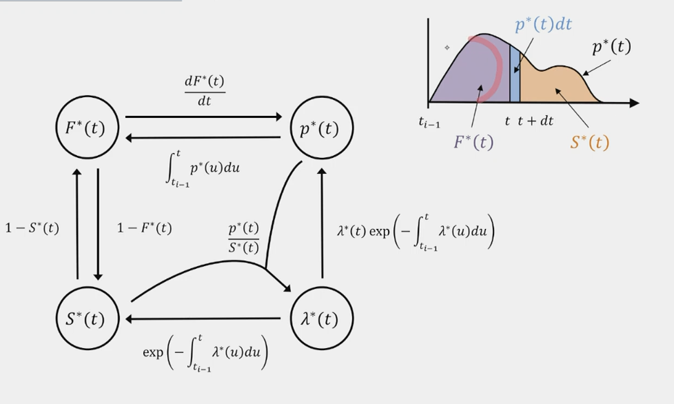
- The next event in \([t, t + dt]\) is \(p^*(t) \, dt\) and there is no event before \(t\)
Conditional Density:
Cumulative distribution function (CDF): \[ F^*(t) = \int_{t-1}^t p^*(t) \, dt \] Probability that the next event is between \(t-1\) and \(t\)
Survival function: \[ S(t) = 1 - F^*(t) = \int_t^\infty p^*(t) \, dt \] Probability that the next event is after \(t\)
Conditional intensity function: \[ \lambda(t) = \frac{p^*(t) \, dt}{S^*(t)} = \frac{P(\text{event in } [t, t + dt] \text{ and no event in } [t-1, t])}{P(\text{no event in } [t-1, t])} \] Probability of the next event in \([t, t + dt]\) given that there is no event in \([t-1, t]\)
- Intuitive interpretation: Number of expected events per unit of time
- Not a probability
The likelihood of the entire sequence with \(t_1, t_2, \ldots, t_n\) events on \([0, T]\) is:
\[ p(t_1, t_2, \ldots, t_n) = p^*(t_1) \cdot p^*(t_2) \cdots p^*(t_n) S^*(T) = \lambda(t_1) \lambda(t_2) \cdots \lambda(t_n) \exp \left( - \int_0^T \lambda^*(t) \, dt \right) \]
\[ p^*(t_1) = \lambda(t_1) \exp \left( - \int_0^{t_1} \lambda^*(t) \, dt \right) \]
Challenges:
- We don’t like the integral
- The number of events can vary
Models Based on Conditional Intensity Functions
- More flexible and interpretable
- Easy to combine different TPPs with different \(\lambda^*(t)\) to produce a new TPP
- Efficient sampling
Homogeneous Poisson Process (HPP)
- Simplest possible model
- \(\lambda^*(t) = \mu\)
- \(p^*(t) = \mu \exp(-\mu (t - t_1))\) is an exponential distribution
We can interpret it as modeling the inter-event times that are exponentially distributed.
Sampling:
- Generate an exponential random variable with rate \(\mu\) and add it to the last event time
- It doesn’t depend on the history (memoryless property), so we can sample all events at once
Inhomogeneous Poisson Process (IPP)
- Intensity function is time-dependent: \(\lambda^*(t) = \mu(t) \geq 0\)
- Still doesn’t depend on the history (memoryless property)
- Captures global trends (e.g., cars on the road during rush hour)
Expected Number of Events:
\[ N([a, b]) \sim \text{Poisson} \left( \int_a^b \mu^*(t) \, dt \right) \]
Simulating an IPP:
- Simulating inter-event times is hard and requires integration
- Better alternative: Thinning algorithm
- Find the upper bound of the intensity function \(\lambda^*(t) \geq \max_t \mu(t)\)
- Sample a time \(t\) from an HPP with rate \(\lambda^*\)
- Accept \(t\) with probability \(\mu(t) / \lambda^*\)
- Essentially acceptance-rejection sampling
Hawkes Process
- Self-exciting process
- Example: Tweets, where one tweet triggers another, then a pause until another tweet
\[ \lambda(t) = \mu + \alpha \sum_i k_w(t - t_i) \quad \text{where } t_i < t \]
- Triggering kernel: \(k_w(t - t_i) = \beta \exp(-\beta (t - t_i)) \text{ for } t > t_i\)
- Parameters: \(\mu, \alpha, \beta\)
- Depends on the history
- Exhibits clustered, bursty behavior
Parameter Estimation in TPPs
- Maximize the likelihood of the observed data over the parameters (iid learning setting)
\[ \log P(t_1, t_2, \ldots, t_n) = \sum_i \log \lambda^*(t_i) - \int_0^T \lambda^*(t) \, dt \]
- Various optimization algorithms
- Simple models like HPP allow for closed-form solutions
- For Hawkes, we can use convex optimization
- We can use gradient descent with modifications for constraints
Advantages and Disadvantages of Using Intensity:
- Numerical integration might be intractable
- Not clear how to define flexible models with arbitrary dynamics
- Easy to interpret, sample, and define models with simple dynamics
We will revisit RNNs with conditional probability.
Directly Model the Conditional Density \(p^*(t \mid H_t)\) with an RNN:
- Every time an event happens, we feed \(\tau_i = t_i - t_{i-1}\) to the RNN
- Use the hidden state to model the history
- Use it to model the parameters of the \(p^*\) distribution
- \(p^*_t = p(t \mid H_t) = p(t \mid h_i)\)
How to Model \(p^*\):
- Simple non-negative distributions: Exponential, Gamma, Weibull, Gompertz
- Use a mixture of distributions: Convex combinations of densities
- If we pick the exponential distribution, it’s not an HPP nor an IPP since it depends on the history and the parameter \(\mu\) changes over time
Normalizing Flows:
- Use transformations like \(\exp(\log(1 + \exp))\) to ensure that the output is positive, combine with other transformations to get a flexible distribution
Problems with Autoregressive TPPs:
- Error accumulation
- Computational complexity
- Hard to model long-range interactions
Alternative: ADD and THIN - Diffusion for TPPs
- Noising: Data sample \(t_0 \sim \lambda_0\)
- For every diffusion step \(n\):
- Thin \(t_{n-1}\) = randomly remove events from data
- Add events from HPP superposed with the history
- End up with completely noised data according to the HPP
- End: Noised data \(\tilde{t}_n \sim \lambda_{\text{HPP}}\)
- Learn the denoising process
- Now we take the entire sequence into account, not autoregressive
Marked TPPs
- Most common type: Categorical mark (type of tweet)
- Each event has a category
- Events of different classes can influence each other
- We can have a distribution over the types: The hidden state can be used to model the type represented by a categorical distribution