Neural Networks
Modern approaches to handling sequential data are increasingly based on neural networks. In this section, we will discuss some of the most popular neural network architectures for sequential data.
Word Vectors
We aim to represent words as vectors.
One-Hot Encoding
One-hot encoding is a simple method but has significant limitations: - There is no relationship between the vectors of different words. - The approach does not scale well with the vast number of words and their forms.
Distributional Hypothesis
According to the distributional hypothesis, words that appear in similar contexts tend to have similar meanings. This means that: - Similar words have vectors near each other. - For example, “hotel” and “motel” can be interchangeable. - However, polysemy can cause issues; for instance, “duck” as an animal and “duck” as a verb would have the same vector despite different meanings.
Illustration: - “king” + “woman” = “queen”
Co-Occurrence Matrix
A co-occurrence matrix captures how often words appear together within a window of size \(l\) around \(x_i\): \(\{x_{i-l}, x_{i-l+1}, \ldots, x_{i+l}\}\). - The co-occurrence matrix \(M\) is of size \(V \times V\) and is typically sparse. - It remains high-dimensional, so dimensionality reduction techniques are often applied. - The matrix is usually normalized by the frequency of the words.
Word2Vec
Word2Vec offers a different way to generate word vectors, as introduced by Mikolov et al. in 2013.
Continuous Bag of Words (CBOW)
- Predicts the target word given context words.
- Not effective for rare words.
Skip-gram
- Predicts context words given a target word.
- Slower to train but can perform better for rare words and small datasets.
- Input: one-hot encoded word vector of size \(N\).
- Embedding: projects into a \(D\)-dimensional space.
- The \(i\)-th row of the embedding matrix (\(N \times D\)) provides the word vector.
- A matrix \(W\) of size \(D \times N\) is used to get the surrounding words.
- Model parameters: \(U\) and \(V\).
- Objective: maximize \(E(P(C|w, U, V))\), where \(C\) is the context word and \(w\) is the target word.
- \(P(C|w, U, V) = \prod P(C_i|w, U, V)\), and \(P(C_i|w, U, V) = \text{softmax}(w_i^T \cdot U \cdot V)_i\).
- \(U\) and \(V\) can be chosen to be the same.
- This results in a dot product between the target word and the context word.
- \(u\) is the embedding.
Training
- Each forward pass computes normalized probabilities over all words, which is inefficient for large vocabularies.
- Alternative: negative sampling.
- Transforms the problem into a binary classification task.
- Samples \(k\) negative words and one positive word.
- Objective: maximize the probability of the positive word and minimize the probability of the negative words.
- Uses sigmoid instead of softmax.
Note: This method ignores the order of words.
Recurrent Neural Networks (RNNs)
In word embeddings, we learn representations for individual words. To process a sequence of words with variable length, RNNs use word embeddings as input and process the sequence one word at a time.
Weight Sharing
- RNNs share weights across all time steps.
- Multiple layers of RNNs can be stacked on top of each other.
Definitions
Given a sequence of words \(x_1, x_2, \ldots, x_t\) and outputs \(y_1, y_2, \ldots, y_t\), we want to compute the probability \(P(y_i | x_1, x_2, \ldots, x_i)\). - A sequence \(x_1\) to \(x_{t-1}\) is represented by a hidden state \(h_{t-1}\). - The network takes \(h_{t-1}\) and \(x_t\) to produce \(h_t\), from which we predict \(y_t\).
Equations: \[ z_t = W_h h_{t-1} + W_x x_t + b \] \[ h_t = \tanh(z_t) \] \[ o_t = V h_t + c \] \[ y_t = \text{softmax}(o_t) \]
The network is fully differentiable, allowing backpropagation through time (BPTT).
Loss: \[ L = - \sum \log P(y_i | x_1, x_2, \ldots, x_i) \]
Backpropagation Through Time (BPTT)
\[ \frac{\partial L}{\partial V} = \sum (y_t - \hat{y}_t) h_t^T \] Since parameters are shared, the final derivative is a sum of all contributions: \[ \frac{\partial L}{\partial h_t} \text{ is a function of } h_{t+1} \text{ and depends on the future.} \] \[ \frac{\partial L}{\partial h_t} = \sum_{s=t}^N \frac{\partial L}{\partial h_s} \frac{\partial h_s}{\partial h_t} = \sum \ldots \prod W \] - If \(W\) has eigenvalues larger than 1, the gradient will explode; if smaller than 1, it will vanish. - RNNs struggle to retain information for long sequences.
Gated Recurrent Unit (GRU)
GRUs modify the architecture to retain information longer by using a gating mechanism.
Equations: \[ z_t = \sigma(W_z[h_{t-1}, x_t]) \] \[ r_t = \sigma(W_r[h_{t-1}, x_t]) \] \[ \hat{h}_t = \tanh(W_h[r_t \odot h_{t-1}, x_t]) \] \[ h_t = (1 - z_t) \odot h_{t-1} + z_t \odot \hat{h}_t \]
- If \(r_t = 0\), the previous state is ignored.
- If \(z_t = 0\), the new state is ignored.
- The gates mix the previous and new states as needed.
Long Short-Term Memory (LSTM)
LSTMs, invented by Hochreiter and Schmidhuber in 1997, use three gates: input, forget, and output.
Equations: \[ i_t = \sigma(W_i[h_{t-1}, x_t]) \] \[ f_t = \sigma(W_f[h_{t-1}, x_t]) \] \[ o_t = \sigma(W_o[h_{t-1}, x_t]) \] \[ \tilde{c}_t = \tanh(W_c[h_{t-1}, x_t]) \] \[ c_t = f_t \odot c_{t-1} + i_t \odot \tilde{c}_t \] \[ h_t = o_t \odot \tanh(c_t) \]
LSTMs maintain both short-term (cell state) and long-term (hidden state) memories. This structure allows for better gradient flow and alleviates the vanishing gradient problem, although training can still be challenging.
Non-Recurrent Models (ConvNets and Transformers)
Sometimes, the full history of a sequence is not needed. Recall autoregressive models, which use a fixed window of the past. While RNNs share parameters across all time steps and depend on the full history, non-recurrent models provide alternative approaches.
Convolutional Neural Networks (ConvNets)
ConvNets can process sequences using convolutions.
- In 2D, convolutions use a filter that slides over the image.
- For sequences, we use 1D convolutions.
- WaveNet, for example, uses dilated convolutions to increase the receptive field, adding gaps between the filter elements to ensure causality. This ensures that the output at time \(t\) only depends on the past.
ConvNets are easier to train and parallelize, with predictions at each time step happening in parallel.
Transformers
Transformers use learned weighting of each element in the sequence instead of fixed weighting, as in convolutions.
Cross-Attention
Inputs: - \(X\): The query, representing the English sentence to be translated. - \(X'\): Both the key and value, representing the German sentence.
Mechanism: - The attention mechanism identifies important parts of \(X'\) (German sentence) for translating \(X\) (English sentence).
Attention Calculation: 1. Deriving Queries, Keys, and Values: - Queries (\(Q\)) are derived from \(X\) (English sentence). - Keys (\(K\)) and Values (\(V\)) are derived from \(X'\) (German sentence).
- Calculating Attention Scores:
- Attention scores are the dot product of queries (\(Q\)) with the transpose of keys (\(K^T\)).
- Scores are scaled by the square root of the dimensionality of the keys (\(d_k\)) for stability.
- Softmax is applied to these scaled scores to obtain attention weights: \[ \text{Attention Weights} = \text{Softmax}\left(\frac{QK^T}{\sqrt{d_k}}\right) \]
- Computing the Weighted Sum:
- Attention weights compute a weighted sum of the values (\(V\)), resulting in the final attention output (\(z\)): \[ z = \text{Attention Weights} \times V \]
Result: - The output \(z\) is an updated representation of \(X\) (English sentence) incorporating relevant information from \(X'\) (German sentence).
Self-Attention
- \(X\) and \(X'\) are the same.
- Self-attention examines relationships between words within the same sentence, acting as a generalized convolution with a data-dependent kernel for the entire sequence.
Positional Encoding
- Attention mechanisms are permutation equivariant, meaning they do not inherently capture word order.
- Positional encoding, often a Fourier transform of the position, addresses this limitation by adding position information to the embeddings.
Multi-Head Attention and Complexity
- Multi-head attention combines the output of \(h\) self-attention heads.
- Each head has its parameters, and their outputs are concatenated and linearly transformed to reduce dimensionality.
- Each head computes \(n^2\) attention scores, making this approach intractable for long sequences.
- Solutions include fixing the structure of attention weights, low-rank approximations, and downsampling the sequence length.
Structured State Space Models (S4)
State Space Model Basics
A discrete-time state space model is defined by the following equations:
\[ \begin{aligned} x_{k+1} &= \mathbf{A}x_k + \mathbf{B}u_k \\ y_k &= \mathbf{C}x_k + \mathbf{D}u_k \end{aligned} \]
Where: - \(x_k \in \mathbb{R}^N\) is the state vector - \(u_k \in \mathbb{R}\) is the input - \(y_k \in \mathbb{R}\) is the output - \(\mathbf{A} \in \mathbb{R}^{N \times N}\), \(\mathbf{B} \in \mathbb{R}^N\), \(\mathbf{C} \in \mathbb{R}^{1 \times N}\), \(\mathbf{D} \in \mathbb{R}\) are the model parameters
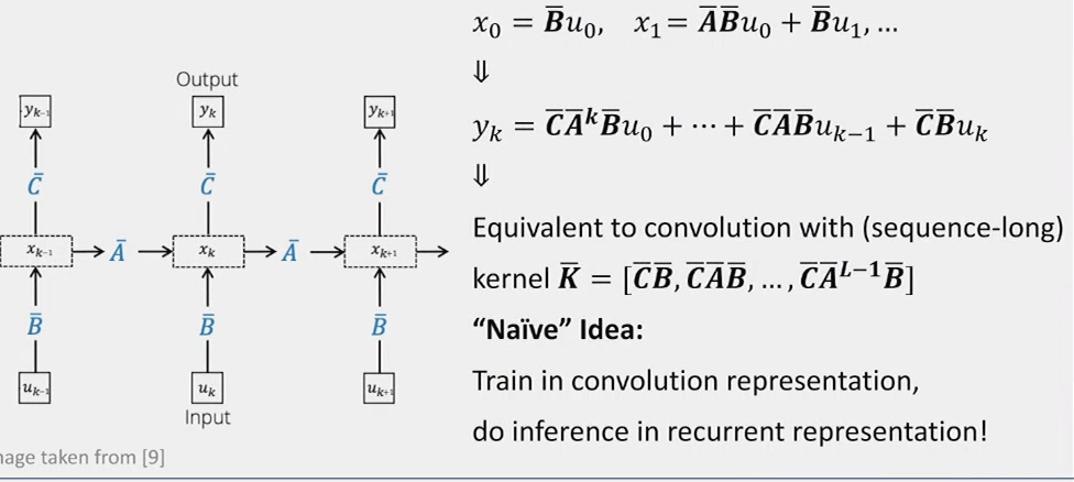
Recurrence as a Convolution
By recursively applying the state equation, we can express the output as a convolution:
\[ \begin{aligned} x_0 &= \mathbf{B}u_0 \\ x_1 &= \mathbf{A}\mathbf{B}u_0 + \mathbf{B}u_1 \\ y_k &= \mathbf{C}\mathbf{A}^k\mathbf{B}u_0 + \mathbf{C}\mathbf{A}^{k-1}\mathbf{B}u_1 + \cdots + \mathbf{C}\mathbf{B}u_{k-1} \end{aligned} \]
This is equivalent to a convolution with a sequence-length kernel:
\[y = K * u, \text{ where } K = [\mathbf{C}\mathbf{B}, \mathbf{C}\mathbf{A}\mathbf{B}, \mathbf{C}\mathbf{A}^2\mathbf{B}, \ldots]\]
Computational Complexity
The naive implementation has a complexity of \(O(N^2L)\) for a sequence of length \(L\), which is impractical for long sequences.
Efficient Computation
To reduce complexity, we can diagonalize \(\mathbf{A}\):
\[\mathbf{A} = \mathbf{V}\boldsymbol{\Lambda}\mathbf{V}^{-1}\]
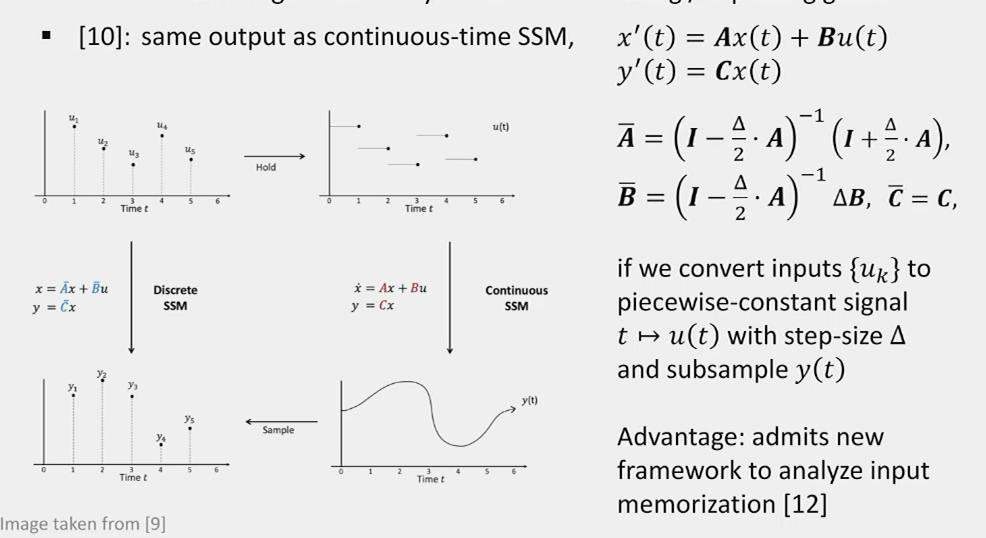
Continuous Time View and HIPPO Initialization
To address the vanishing/exploding gradient problem, we can use a continuous-time perspective:
\[\frac{d}{dt}x(t) = \hat{\mathbf{A}}x(t) + \hat{\mathbf{B}}u(t)\]
The discrete-time \(\mathbf{A}\) is related to the continuous-time \(\hat{\mathbf{A}}\) by:
\[\mathbf{A} = e^{\Delta \hat{\mathbf{A}}}\]
Where \(\Delta\) is the step size.
The HIPPO (HIerarchical Positive Orthogonal) initialization sets \(\hat{\mathbf{A}}\) to a specific form that ensures stable gradient flow and long-term memory. It’s based on the recurrence relation of Legendre polynomials.
Legendre Polynomials (LP)
The nth Legendre polynomial \(P_n(x)\) satisfies:
\[(2n+1)xP_n(x) = (n+1)P_{n+1}(x) + nP_{n-1}(x)\]
This recurrence relation allows efficient updates of the state as new data points are added.
S4: Structured State Space for Sequences
The S4 model combines these elements:
- HIPPO initialization of \(\hat{\mathbf{A}}\)
- Efficient kernel computation using the diagonalization trick
- Multiple layers with non-linearities (e.g., ReLU) between them
- Residual connections: \(y^{(l)} = u^{(l)} + \text{S4}(u^{(l)})\)
The full S4 layer can be expressed as:
\[\text{S4}(u) = \phi(K * u + b)\]
Where \(\phi\) is a non-linearity and \(b\) is a bias term.
S4 has achieved state-of-the-art performance on various long-range sequence modeling tasks, outperforming traditional RNNs and even Transformers in some cases.