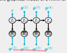
Hidden Markov Models
Basic Markov Models are very restrictive/simple and do not capture the complexity of the real world.
Probabilistic latent variable models for a sequence of observations: \(X_1 \rightarrow X_2 \rightarrow X_3 \rightarrow ... \rightarrow X_t\)
We use discrete time steps, while observations can be continuous or discrete.
Examples: - \(X_t\): location of a moving object - \(X_t\): word in a sentence
In many applications, the Markov property is not realistic as we have long dependencies. \(X_t\) does not capture all relevant information.
In many applications, the state is not directly known but can only be observed indirectly with sensor data. Markov Chain is a fully observed model - not realistic.
Example: Tracking a plane - Not observed/latent state \(Z_t\): physical vector quantities (position, velocity, acceleration) - \(X_t\): observed noisy measurements of the state (radar, GPS, etc.) - \(Z_t\) has the Markov property; one can approximate the state of the plane at time \(t\) given the state at time \(t-1\) - \(X_t\) doesn’t have to have the Markov property
Definition
A sequence of latent states \(Z_1, Z_2, ..., Z_t\) and observations \(X_1, X_2, ..., X_t\) where: - \(Z_t\) is a Markov chain - \(X_t\) is conditionally independent of all other states given \(Z_t\) - \(P(X_t | Z_1, Z_2, ..., Z_t, X_1, X_2, ..., X_{t-1}) = P(X_t | Z_t)\) - Distribution of \(X_t\) depends only on the current state \(Z_t\) - We assume discrete time and discrete latent states \(Z_t\) -> we can treat it as a Markov chain with a transition matrix \(A\) - \(X_t\) can be continuous or discrete
\[P(X_1, X_2, ..., X_t, Z_1, Z_2, ..., Z_t) = P(Z_1)P(X_1 | Z_1)P(Z_2 | Z_1)P(X_2 | Z_2) ... P(Z_t | Z_{t-1})P(X_t | Z_t)\]
\(P(Z_1 = i) = \pi_i\)
\(P(Z_t = j | Z_{t-1} = i) = A_{ij}^{t+1}\)
\(P(X_t = j | Z_t = i) = B_{ji}^{t+1}\)
\(A\) is \(K \times K\)
\(B\) is \(K \times M\) where \(M\) is the number of observed states
Too many parameters, we assume time homogeneous model
Tasks
Parameter estimation: Observed \(X_1, X_2, ..., X_t\) -> estimate \(\pi, A, B\) and the most likely sequence of states \(Z_1, Z_2, ..., Z_t\)
Inference:
- Filtering: Infer \(Z_t\) given \(X_1, X_2, ..., X_t\) (online) - predict the location of a robot
- Smoothing: Infer \(Z_t\) given \(X_1, X_2, ..., X_T\) (offline) given all observations - predict the stem of a word in a sentence
- MAP inference: Infer the most likely sequence of states given the observations
- \(\arg\max_z P(Z_1, Z_2, ..., Z_t | X_1, X_2, ..., X_t)\)
- Mode of the posterior distribution
- Viterbi decoding
- Attention: Most probable sequence might be different than using smoothing per each time step
Filtering: Forward Algorithm
\[P(Z_t | X_1, X_2, ..., X_t) = \frac{P(X_1, X_2, ..., X_t, Z_t)}{P(X_1, X_2, ..., X_t)} = \frac{P(X_1, ..., X_t, Z_t)}{\sum_{Z_t} P(X_1, X_2, ..., X_t, Z_t)}\]
\(\alpha_t(i) = P(X_1, X_2, ..., X_t, Z_t = i)\) Vector of size \(K\)
\[P(Z_t | X_1, X_2, ..., X_t) = \frac{\alpha_t(i)}{\sum_i \alpha_t(i)}\]
Efficient computation of \(\alpha_t(i)\): - Recursive - \(\alpha_1(i) = P(X_1, Z_1 = i) = P(Z_1 = i)P(X_1 | Z_1 = i) = \pi_i B_{ix_1}\) - \(\alpha_{t+1}(k) = P(X_1, X_2, ..., X_{t+1}, Z_{t+1} = k)\) \(= P(X_{t+1}|X_{1:t}, Z_{t+1} = k)P(X_{1:t}, Z_{t+1} = k)\) \(= P(X_{t+1}|Z_{t+1} = k) \sum P(Z_{t+1} = k, Z_t = i, X_{1:t})\) \(= P(X_{t+1}|Z_{t+1} = k) \sum P(Z_{t+1} = k | Z_t = i)P(Z_t = i, X_{1:t})\) \(= B_{kx_{t+1}} \sum A_{ij} \alpha_t(i)\)
\(\alpha_{t+1} = B_{x_{t+1}} \cdot (A^T \alpha_t)\) \(O(K^2T)\) which is linear in \(T\)
The Forward-Backward Algorithm: Smoothing
We have seen the entire data sequence \(X_1, X_2, ..., X_T\) \[P(Z_t | X_{1:T}) = \frac{P(X_{1:T}, Z_t)}{P(X_{1:T})} = \frac{P(X_{1:t}, Z_t = k) P(X_{t+1:T}| Z_t = k)}{\sum_{Z_t} P(X_{1:T}, Z_t)}\]
\(\beta_t(i) = P(X_{t+1:T} | Z_t = i)\) Hence \(P(Z_t | X_{1:T}) \propto \alpha_t(i) \beta_t(i)\) just normalized over \(i\)
Backward algorithm computes recursively: - \(\beta_T\) initialization - Given \(\beta_{t+1}\) compute \(\beta_t\) - \(\beta_T(i) = 1\) (has to be to work out, it doesn’t exist) - \(\beta_t(j) = P(X_{t+1:T} | Z_t = j) = \sum_i P(X_{t+1:T}, Z_{t+1} = i | Z_t = j)\) \(= \sum_i P(X_{t+1}, Z_{t+1} = i | Z_t = j)P(X_{t+2:T} | Z_{t+1} = i)\) \(= \sum_i P(Z_{t+1} = i | Z_t = j)P(X_{t+1} | Z_{t+1} = i)P(X_{t+2:T} | Z_{t+1} = i)\) \(= \sum_i A_{ji} B_{t+1}(i) \beta_{t+1}(j)\)
\(\beta_t = A (B_{x_{t+1}} \cdot \beta_{t+1})\)
\(O(K^2T)\) which is linear in \(T\)
Final Solution
- Compute prob of being in state \(k\) at time \(t\) online: We compute \(\alpha\)
- Compute prob of being in state \(k\) at time \(t\) offline: We compute \(\alpha\) and \(\beta\)
MAP Inference: Viterbi Decoding
\[\arg\max_z P(Z_1, Z_2, ..., Z_t | X_1, X_2, ..., X_t) = \arg\max_z P(X_1, X_2, ..., X_t, Z_1, Z_2, ..., Z_t)\] \[= \arg\max [\log P(Z_1)P(X_1| Z_1) + \sum \log P(Z_t | Z_{t-1}) + \log P(X_t | Z_t)]\]
Bipartite graph with weights: \(-\log P(X_t | Z_t) P(Z_t | Z_{t-1})\) Find the shortest path from the source to the sink
We have \(TK^2\) edges and \(TK\) nodes, so we can use Dijkstra’s algorithm to find it in \(O(TK^2 \log(TK))\)
Parameter Estimation: Learning \(\pi, A, B = \theta\)
Solve \(\max_\theta \sum \log P(X_1, X_2, ..., X_T | \theta)\) No analytical solution due to marginalization Use EM algorithm same as in GMM
GMM is a HMM without dependencies
EM Algorithm for HMM
E-step: Compute \(\alpha\) and \(\beta\) - Evaluate the posterior \(P(Z|X, \theta_\text{old})\)
M-step: Update \(\pi, A, B\) - Maximize the expected joined log likelihood \(P(X, Z | \theta)\) under \(\theta_\text{old}\) - \(\theta_\text{new} = \arg\max_\theta \sum P(Z|X, \theta_\text{old}) \log P(X, Z | \theta)\)
The M-step is equivalent to maximizing the Evidence Lower Bound (ELBO) as in variational inference, which is a lower bound on \(P(X|\theta)\) - We are testing all possible \(Z\)s weighted by the probability of the \(Z\)s
The MLE estimate for parameters is just the expected counts of the transitions and the emissions and the initial state distribution
Additions
Continuous Observations: Gaussian Emissions
\(P(X_t | Z_t = i) = \mathcal{N}(X_t | \mu_i, \sigma_i I)\) It can be used for time series segmentation - \(Z_i\) are clusters of similar behavior - Observations are Gaussians coming from the clusters - Time series emits from one cluster until it switches to another cluster
It is the same as before; we use Viterbi decoding to find the most likely sequence of states
If we had continuous latent states and continuous observations, we could use Kalman filters
Extensions: Neural Hidden MM/Deep State Space Models
\(P(Z_t | Z_{t-1}) = \mathcal{N}(Z_t | f(Z_{t-1}), \sigma_z)\) \(P(X_t | Z_t) = \mathcal{N}(X_t | g(Z_t), \sigma_x)\) There are no constraints on \(f\) and \(g\) They can be NN optimized by gradient descent - in the M-step to get new \(\theta\) - Before we had closed-form solutions We don’t have to use Gaussian distributions
Discussion
We only discuss discrete time steps - it’s essentially just an ordered series In applications: - Asynchronous time - events/measurements can happen with different gaps - speech recognition, temporal point processes - Continuous time - measurements almost continuously, examples: temperature - continuous stochastic processes