Autoregressive Models (AR Models)

Overview

An autoregressive (AR) model is used for modeling and predicting time series data where observations are dependent on previous time steps. Here are the key concepts and components of AR models:

Key Concepts

• Sequence of Observations: \(X_1, X_t\), where \(t\) is a time index, location, etc.
• Continuous Observations: Occur at discrete time steps.
• Applications:
  • Time series forecasting (e.g., temperature, stock prices).
  • Sequence of words in a sentence.
• Dependence: Observations are not independent and identically distributed (not i.i.d.).

AR Model of Order \(p\)

The AR model of order \(p\) is defined as: \[ X_t = c + \sum_{i=1}^{p} \phi_i X_{t-i} + \epsilon_t \] where: - \(\phi_i\) are the parameters of the model. - \(c\) is a constant. - \(\epsilon_t\) is the error term (white noise). - \(X_{t-i}\) is the lagged value of the time series.

Intuitively, the AR model is a linear regression of the current value of the time series on the past \(p\) values.

Long-term Effects

A modification or shock to \(X_t\) will have a long-term effect on the time series.

Regression View

For regression, we can represent the data in matrix form: \[ X = \begin{bmatrix} X_{p-1} & X_{p-2} & \cdots & X_0 \\ X_p & X_{p-1} & \cdots & X_1 \\ X_{p+1} & X_p & \cdots & X_2 \\ \end{bmatrix} \] \[ y = \begin{bmatrix} X_p \\ X_{p+1} \\ X_{p+2} \\ \end{bmatrix} \] The parameters \(\phi\) can be estimated using: \[ \phi = (X^T X)^{-1} X^T y \] or using stochastic gradient descent (SGD) with mean squared error (MSE) loss.

Training

Only one time series is needed to train the model.

Probabilistic View

The probability of \(X_t\) given the past \(p\) values is: \[ P(X_t | X_{t-1}, X_{t-2}, \ldots, X_{t-p}) = \mathcal{N}\left(c + \sum_{i=1}^{p} \phi_i X_{t-i}, \sigma^2\right) \] where: - \(\mathcal{N}\) is the normal distribution. - \(c\) and \(\phi\) are shared across all time steps. - Maximum likelihood estimation (MLE) would be the same as the regression view.

Generative Model

The AR model is also a generative model.

Mean Function

\[ \mu(t) = \mathbb{E}(X_t) \]

Auto Covariance Function

\[ \gamma(t, i) = \mathbb{E}[(X_t - \mu(t))(X_{t-i} - \mu(t-i))] = \text{Cov}(X_t, X_{t-i}) \] - Indicates the dependence between two time steps. - Prediction is not deterministic due to the white noise term.

General Remark: Data Split

• Non-i.i.d Data: We cannot split the data randomly.
• Temporal Split: The model should be trained on past data and tested on future data.
• K-Fold Across Time: Keep the validation set the same size and shift it to the right.

General Remark: Stationarity

A time series is stationary if: - \(\mathbb{E}(X_t) = \mu\) for all \(t\). - \(\text{Cov}(X_t, X_{t-i}) = \gamma(i)\) for all \(t\).

This allows us to estimate \(\mu\) and \(\gamma\) from the data, making it a good modeling assumption.

Parameters

Parameters learned from one part of the time series can be used to predict another part.

Yule-Walker Equations

Assuming stationarity, we can learn the parameters of the AR model using the Yule-Walker equations: \[ \gamma_i = \sum_{t=1}^{p} \phi_t \gamma_{i-t} \] \[ \gamma_0 = \sigma^2 + \sum_{i=1}^{p} \phi_i \gamma(i) \]

• Estimate the moments \(\gamma(i)\) from the data.
• Solve this system of linear equations to get the \(\phi\) parameters.
• Use \(\gamma(0)\) to estimate \(c\) and \(\sigma^2\).

Moment Matching

We use moment matching to estimate parameters.

Questions

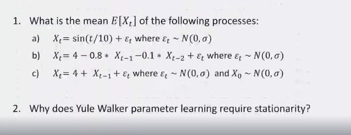
Screenshot of questions