Introduction

Very common modality of data. Includes images and text. General graphs are permutationally invariant and we can place the nodes anywhere in space.

Graph Theory and Network Structure

Basic Definitions

Plain Simple Graph $G = (V, E)$: - Set of nodes $V$ - Set of edges $ E V V$ - For undirected graphs, $(u, v) = (v, u)$ - Equivalent representation: adjacency matrix $A \in \{0, 1\}^{|V| \times |V|}$ - Extensions: weighted, attributed (vectors assigned to nodes or edges), temporal

Structure of Real Networks

Are Real Networks Random? - No, they are not random.

Erdős–Rényi Model: - Random graph model - Start with $n$ nodes - For each pair of nodes, add an edge with probability $p$ - Every edge is independent - No obvious pattern - Not a good model for real networks

Interpretation Challenges: - We cannot interpret the adjacency matrix directly nor plot it. - When plotting graphs, we use a layout algorithm that changes how the graph looks - graph isomorphism.

Patterns in Real Graphs

Diameter: - Very small, following the “six degrees of separation” concept.

In-degree and Out-degree Distribution: - Follows a power law. - Few nodes have many connections, and many nodes have few connections. - Log-log plot looks like a straight line. - The decay of the probability density function (pdf) is polynomial, not exponential (heavy-tailed): \[ p(x) = a \cdot x^{-b} \quad \text{where } b > 1 \] - Graphs with power law degree distribution are called .

Scale-free Property: - The number of nodes with degree $x$ is denoted by $y(x)$. - For a scale-free network, the degree distribution follows a power law: \[ y(x) \propto x^{-b} \] - Here, $y(x)$ is the number of nodes with degree $x$. - $a$ and $b$ are constants, with $b > 1$.

Scale-free Property Equation: - The scale-free property suggests that the degree distribution is invariant under rescaling: \[ y(ax) = a^{-b} y(x) \] - This means that if you scale the degree by a factor $a$, the number of nodes with that degree scales by a factor $a^{-b}$.

Algorithm Design Considerations

We need to account for power law distributions when designing algorithms.
Gaussian assumptions often do not hold (Gaussian trap).

Clustering Coefficient: - Calculated as $\frac{3 \times \text{number of triangles}}{\text{number of connected triples}}$ - Real graphs have a large clustering coefficient, indicating strong community structure.

Approximating the Clustering Coefficient

Plot the sorted eigenvalues of the adjacency matrix on a log-log plot.
Power law distribution: few large eigenvalues and many small ones.
Number of triangles: \[ \text{Number of triangles} = \frac{\text{trace}(A^3)}{6} = \frac{\sum (\text{eigenvalues}^3)}{6} \]
We only need the largest eigenvalues, which can be computed efficiently using the power iteration method:
- Multiply a random vector with the matrix and normalize it.
- Converges to the largest eigenvector.
- Deflated matrix $\hat{X} = X - \lambda_1 v_1 v_1^T$ (works only for symmetric matrices).

Sparsity of Real Graphs: - While there are $N^2$ possible edges, the real number of edges is almost linear.

Path Lengths and Diameters

Characteristic Path Length: - Median of the average shortest path length between all pairs of nodes.

Average Diameter: - Average of the average shortest path length between all pairs of nodes.

Hop Plots: - $N_h(u)$: Number of nodes reachable from $u$ via $h$ hops. - Total neighbors $N_h$: Sum of all $N_h(u)$ over all $u$. - Plot $N_h$ vs. $h$.

Effective Diameter/Eccentricity: - Minimum number of hops in which a certain fraction (typically 90%) of all connected pairs of nodes can be reached: \[ \min \{ h \mid N_h \geq 0.9 \times \text{total number of reachable pairs} \} \]

Detecting Abnormal Behavior

Understanding what is normal helps in detecting abnormal behavior.
Use realistic graph generators to simulate networks.

Generative Models

Generate graphs with specific properties.

Erdős–Rényi Model

Random graph model:
- Start with $n$ nodes.
- For each pair of nodes, add an edge with probability $p$.
- Every edge is independent.
- No obvious pattern.
- Not a good model for real networks.
$A_{ij} \sim \text{Bernoulli}(p)$
Degree distribution is binomial:
- Probability of having degree $k$: \[ p_k = \binom{n}{k} p^k (1-p)^{n-k} \]
- Can be approximated as Poisson.
Diameter: \[ \text{Diameter} \approx \frac{\log(n)}{\log(z)} \] where $z$ is the average degree.
- Grows slowly with $n$ but in real data, we observe a small constant or even shrinking diameter.
Clustering coefficient:
- Needs specification in this model.

Planted Partition Model

Two communities:
- Each node has a community.
- $p_{\text{intra}}$: Probability of edge within the community.
- $p_{\text{inter}}$: Probability of edge between communities.
Latent variable model: It’s not iid - we condition on two community labels. \[ P(A_{ij} = 1 \mid z_i, z_j) = \begin{cases} p_{\text{intra}} & \text{if } z_i = z_j \\ p_{\text{inter}} & \text{if } z_i \neq z_j \end{cases} \]
Can generalize to weighted and directed edges.

Stochastic Block Model

$k$ communities:
- Generalizes PPM to graphs with $k$ communities and varying edge densities.
- $z_i$: Node $i$ belongs to community $z_i \in \{1, ..., k\}$.
Model parameters:
- $p_i$: Community proportion.
- $p_{ij}$: Edge probability between communities $i$ and $j$.
- $P(z_i = i) = p_i$
- $P(A_{ij} = 1 \mid z_i, z_j) = p_{ij}$
- $\eta$: Transition matrix.

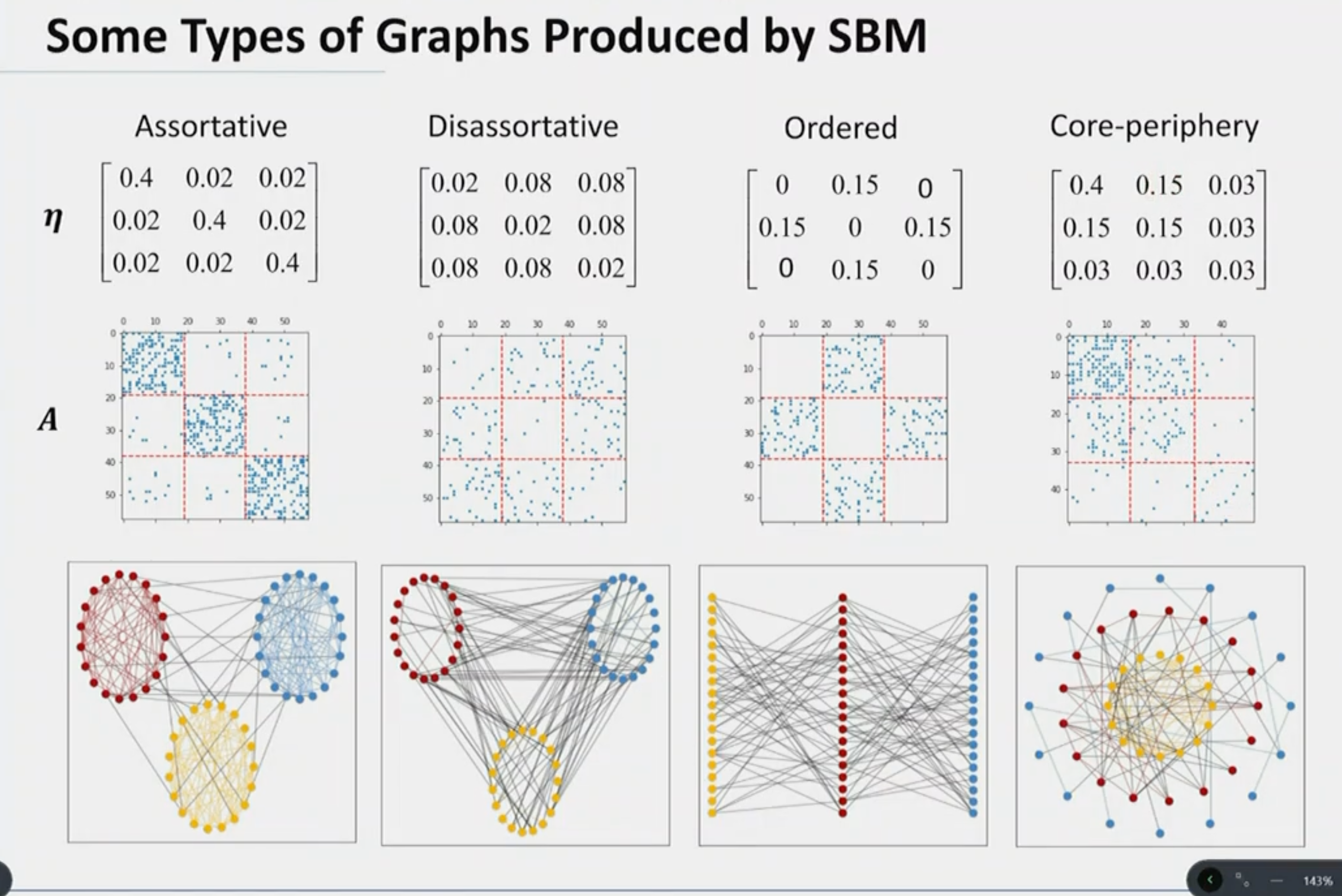
Doesn’t capture all patterns of real networks:
- Degree-corrected SBM.
- Real networks have more triangles: Geometric SBM.
- Real communities are overlapping: Community affiliation graph model.

Preferential Attachment Model

EP/PPM/SMB assume that edges are formed independently.
Start with a small number of nodes and let it grow by adding nodes and edges.
Preferential attachment: New nodes prefer to connect to nodes with high degree (rich get richer - power law degree distribution).

Initial Attractiveness: - Can realize power law with exponent in $[2, \infty]$.

Algorithm: 1. Start with $m_0$ nodes. 2. Add a new node $w$. 3. Add $m$ directed edges $(u, v)$. 4. Probability that the endpoint of an edge $(u, v)$ corresponds to $v$ is proportional to current degree + IA: \[ A_v = A + \text{in-degree}(v) \] where $A$ is the initial attractiveness (same for all nodes). 5. Not important where the edge starts; they can all start from $w$ or existing nodes. 6. Repeat from step 2.

Parameters: - $m, A$ - Degree distribution: \[ \gamma = 2 + \frac{A}{m} \] - Matches many real networks. - Diameter grows logarithmically with $n$. - Average degree remains constant.

Configuration Model

Given a degree sequence, generate a graph:
- Assign a degree to each node represented as a stub (a half-edge).
- Randomly pair the stubs.

Deep Generative Models

Learn models from data:
- All previous models are handcrafted.
- More flexible.
Methods: VAE, GAN, Normalizing Flows, Score-based models, Denoising Diffusion (chronological order of development).
Example: NetGAN - latent space interpolations produce smoothly changing graphs.
- Sample from noise.
- Manipulate the latent space to generate graphs with specific properties.

Ranking

PageRank

Core Idea: A page is important if many important pages link to it, based on a recursive formulation.

Voting Principle: - Each page votes on the importance of pages it links to. - A link’s vote is proportional to the importance of its source page. - If page $j$ with importance $r_j$ has $n$ out-links, then each link gets $\frac{r_j}{n}$ votes. - A page’s own importance is the sum of the votes on its in-links: \[ r_j = \sum_{i} \frac{r_i}{d_i} \] where $i$ links to $j$ and $d_i$ is the out-degree of $i$.

This is a system of linear equations with an infinite number of solutions. We normalize the sum of $r_j$ to 1. For large systems, iterative methods are used.

Stochastic Adjacency Matrix: - $M_{ji}$: If $i$ links to $j$ then $\frac{1}{d_i}$, else 0. - This is a column stochastic matrix, which does not have negative eigenvalues.

Rank Vector: - The rank vector $r$ sums to one and is $\geq 0$: \[ r = Mr \] \[ r = (I - M)^{-1} \cdot e \] - This is an eigenvector problem with eigenvalue 1: \[ ||Mr|| = 1 \] - We find the largest eigenvector of $M$ using power iterations, which converge quickly.

Interpretations: - System of linear equations. - Eigenvector problem. - Fixed point problem. - Random walk.

Random Walk Interpretation

Forms a Markov chain: - At time $t$, the walker is on a random page $i$. - At time $t+1$, the surfer follows an out-link $j$ with probability $\frac{1}{d_i}$.

Transition Matrix: $B = M^T$ - The stationary distribution of $B$ is the PageRank vector: \[ r = rB \] - The initial distribution does not matter: \[ P(X_t = i) = \pi_i(t) \]

Limiting Distribution: - $\pi$ is the limiting distribution if we do infinite steps: - Irreducible: We can get from every state to every other state. - Aperiodic: No cycles (state $i$ is aperiodic if the GCD of all cycle lengths is 1; if one node is aperiodic and irreducible, all nodes are aperiodic).

PageRank score indicates the probability of being on a page after infinite steps—visiting more often means greater importance.

Problems: - Dead ends: No out-links, causing importance to leak. - Spider traps: A set of pages that link to each other but not to the outside. - Periodic states: Cycles.

Solutions: - Random teleportation: At each step, the surfer has two options: - Follow a link with probability $\beta$. - Teleport to a random page with probability $1 - \beta$: \[ r_j = \beta M_{ji} + \frac{1 - \beta}{N} \] - This forms a fully connected matrix: \[ A = \beta M + (1 - \beta) ee^T \frac{1}{N} \] - Instead of full matrix multiplication, we multiply by $M$ and then add the teleportation part, keeping only the vector: \[ r = \beta Mr + \frac{1 - \beta}{N} e \]

Vertex-Oriented Computation: - Each vertex computes a local operation. - Special systems: GraphLab, Giraph, GraphX. - GAS principle: Gather, Apply, Scatter (for PageRank, only Gather and Apply are needed).

This does not solve the issue of dead ends, where the jumping probability becomes 1.

Other Problems: - Measures generic popularity: Biased against topic-specific authorities. - Topic-sensitive PageRank: Evaluates how important a page is for a specific topic, allowing search queries to be answered based on user interests. This involves: - Biasing the random walk. - Picking a set of seed pages $S$ (topic-relevant pages) and teleporting only to them. - Defining $v$ with $\frac{1}{|S|}$ on the columns of the seed pages: \[ r = \beta Mr + (1 - \beta) v \] \[ r = (1 - \beta) (I - \beta M)^{-1} v \] - Personalized PageRank: $v$ has a 1 on your page and 0 on the rest.

Susceptible to Link Spam: - Artificial links increase importance. - TrustRank: Use a set of trusted pages and teleport to them to avoid farmed links.

Uses a Single Measure of Importance: - HITS (Hyperlink Induced Topic Search): - Authority: Pages that are linked to by many hubs. - Hub: Pages that link to many authorities.

Clustering

We can utilize the graph structure to extract clusters without needing any features. These clusters can be later interpreted with some prior knowledge.

Main Idea: There are many edges within clusters and few edges between clusters, leading to high intra-cluster density and low inter-cluster density.

Categories of Clustering Algorithms

Partitioning Methods: Divide the graph into non-overlapping clusters.
Non-Partitioning Methods: Allow clusters to overlap.

Partitioning Methods

Basic Idea: Formulate clustering as a constrained optimization problem.

k-Means with Different Distance Metrics

Given a graph $G$ and an objective: - Define a set of clusters $C = \{C_1, C_2, ..., C_k\}$. - Optimize $G(C)$ subject to $C_1 \cup C_2 \cup ... \cup C_k = V$ and $C_1, C_2, ..., C_k$ are disjoint.

This problem is NP-hard due to its discrete nature. For $k = 2$, polynomial-time algorithms exist.

Global Minimum Cut

Minimize the number of edges between clusters: - Objective: Partition the graph into two clusters such that the cut $(C_1, C_2) = \sum$ of edges between $C_1$ and $C_2$ is minimized. - The source-sink cut can be computed in polynomial time using the Ford-Fulkerson algorithm. - In graph clustering, no specific source and sink are given, and more than two clusters are needed.

Normalized Cut

Cuts tend to favor small clusters.

Ratio Cut: - Minimize $\text{cut}(C_1, C_2) / |C_1| + \text{cut}(C_1, C_2) / |C_2|$. - Does not consider intra-cluster density.

Normalized Cut: - Minimize $\text{cut}(C_1, C_2) / \text{vol}(C_1) + \text{cut}(C_1, C_2) / \text{vol}(C_2)$, where $\text{vol}(C)$ is the sum of the degrees of all nodes in $C$. - For more than two clusters, minimize $\sum_{C_i} \text{cut}(C_i, V \setminus C_i) / \text{vol}(C_i)$. - This is NP-hard; approximate solutions use expectation maximization.

Graph Laplacian - Background

The Graph Laplacian $L = D - W$: - $D$ is the degree matrix. - $W$ is the weighted adjacency matrix. - $L$ is positive semi-definite and symmetric for undirected graphs.

Key Properties: - $f^T L f = \sum_{i,j} W_{ij} (f_i - f_j)^2$ over edges. - The smallest eigenvalue is 0, with the corresponding eigenvector being the constant vector. - The number of connected components is given by the multiplicity of the 0 eigenvalue. - If the graph is connected, the second smallest eigenvalue ($\lambda_2$) is greater than 0. - The second smallest eigenvalue (Fiedler value) indicates the graph’s algebraic connectivity. - The Laplacian is additive under graph union: $L(G_1 \cup G_2) = L(G_1) + L(G_2)$ if $G_1$ and $G_2$ are disjoint.

Normalized/Symmetric Laplacian: - $L_{\text{sym}} = D^{-1/2} L D^{-1/2}$.

Computational Methods: - Spectral clustering involves solving an eigenvalue problem. - For $k = 2$: - Define $f$ such that $f_i = +1$ if $i \in C_1$ and $-1$ if $i \in C_2$. - $f^T L f = 4 \cdot \text{cut}(C_1, C_2)$. - Minimize $f^T L f$ subject to $f^T f = \sqrt{n}$ and $f^T 1 = 0$. - The solution is the second eigenvector of $L$.

For $k > 2$:
- Indicator matrix $H = [h_1, h_2, ..., h_k]$ where $h_j = 1$ if $i \in C_j$ and 0 otherwise.
- $H^T H = I$.
- Minimize $\text{trace}(H^T L H)$.
- The solution is the $k$ smallest eigenvectors of $L$.
Spectral embedding for node $1$ is the first entry of the $k$ smallest eigenvectors of $L$ (first row of $H$).
Perform k-means on the spectral embedding to obtain cluster assignments.

If the weight between nodes in different clusters increases, the spectral embedding will converge.

Drawbacks: There is no guarantee that the approximation will be accurate in all cases, but it works well in practice.

Spectral Clustering for Numerical Data: - Requires a similarity function $ (x,y) = (-||x-y||^2 / 2 ^2)$. - Create an edge between $x$ and $y$ if $\text{sim}(x,y) > t$ or if $x$ and $y$ are mutual $k$-nearest neighbors. - Apply spectral clustering. - Advantages: Works well for non-convex clusters and complex shapes (more effective than applying k-means directly).

Probabilistic Community Detection

Optimization Methods: - Find clustering that minimizes an objective function like min cut.

Generative Models: - Consider a graph as a realization from a generative model controlled by parameters. - Communities are explicitly modeled within the generative model (e.g., PPM, SBM). - Finding good clustering is equivalent to parameter inference.

Example: PPM (Plantinum Partition Model): - Two communities with a latent variable $z$. - Probability $P(A_{ij} = 1 \mid z_j, z_i) = p$ if $z_i = z_j$ and $q$ otherwise. - Maximize the posterior estimate $z^* = \arg \max_z P(Z \mid A)$. - Assume $C_1 = C_2 = n/2$ then $\sum z_i = 0$ (indicator: +1 or -1).

We can show that $P(Z \mid A) \propto P(A \mid Z) = \left( \frac{(1-q)p}{(1-p)q} \right)^{E_{\text{cut}}(z)}$ (if $q > p$), where $E_{\text{cut}}(z) = \sum_{i<j} A_{ij} 1(z_i \ne z_j)$. Minimize the cut to maximize the posterior. This can be solved using spectral clustering for this specific case.

Example: SBM (Stochastic Block Model): - Skip detailed explanation. - Use variational inference to handle intractable posteriors and infer model parameters.