Generative Models
Generate graphs with specific properties.
Erdős–Rényi Model
- Random graph model:
- Start with \(n\) nodes.
- For each pair of nodes, add an edge with probability \(p\).
- Every edge is independent.
- No obvious pattern.
- Not a good model for real networks.
- \(A_{ij} \sim \text{Bernoulli}(p)\)
- Degree distribution is binomial:
- Probability of having degree \(k\): \[ p_k = \binom{n}{k} p^k (1-p)^{n-k} \]
- Can be approximated as Poisson.
- Diameter: \[ \text{Diameter} \approx \frac{\log(n)}{\log(z)} \] where \(z\) is the average degree.
- Grows slowly with \(n\) but in real data, we observe a small constant or even shrinking diameter.
- Clustering coefficient:
- Needs specification in this model.
Planted Partition Model
- Two communities:
- Each node has a community.
- \(p_{\text{intra}}\): Probability of edge within the community.
- \(p_{\text{inter}}\): Probability of edge between communities.
- Latent variable model: It’s not iid - we condition on two community labels. \[ P(A_{ij} = 1 \mid z_i, z_j) = \begin{cases} p_{\text{intra}} & \text{if } z_i = z_j \\ p_{\text{inter}} & \text{if } z_i \neq z_j \end{cases} \]
- Can generalize to weighted and directed edges.
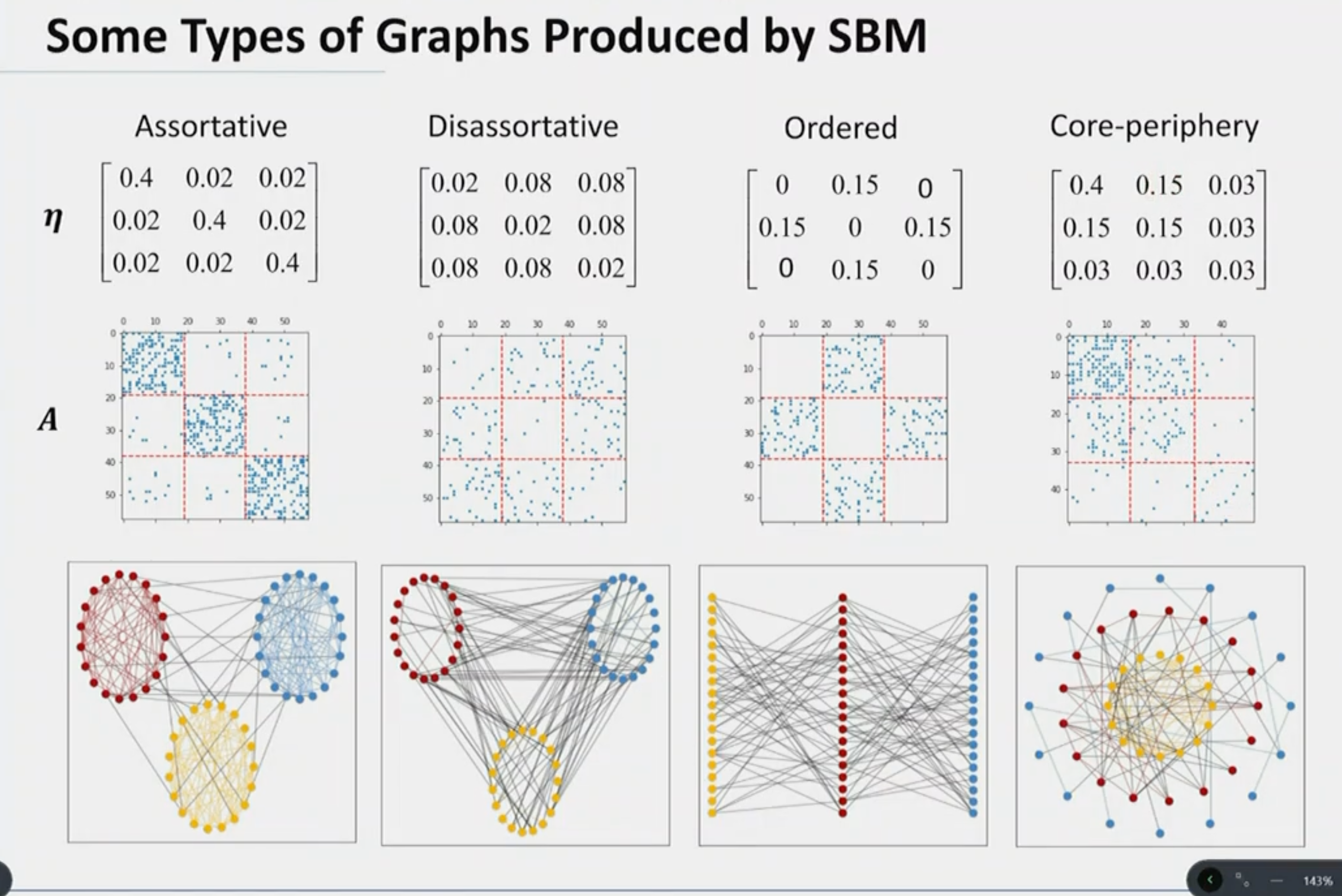
Stochastic Block Model
- \(k\) communities:
- Generalizes PPM to graphs with \(k\) communities and varying edge densities.
- \(z_i\): Node \(i\) belongs to community \(z_i \in \{1, ..., k\}\).
- Model parameters:
- \(p_i\): Community proportion.
- \(p_{ij}\): Edge probability between communities \(i\) and \(j\).
- \(P(z_i = i) = p_i\)
- \(P(A_{ij} = 1 \mid z_i, z_j) = p_{ij}\)
- \(\eta\): Transition matrix.
- Doesn’t capture all patterns of real networks:
- Degree-corrected SBM.
- Real networks have more triangles: Geometric SBM.
- Real communities are overlapping: Community affiliation graph model.
Preferential Attachment Model
- EP/PPM/SMB assume that edges are formed independently.
- Start with a small number of nodes and let it grow by adding nodes and edges.
- Preferential attachment: New nodes prefer to connect to nodes with high degree (rich get richer - power law degree distribution).
Initial Attractiveness: - Can realize power law with exponent in \([2, \infty]\).
Algorithm: 1. Start with \(m_0\) nodes. 2. Add a new node \(w\). 3. Add \(m\) directed edges \((u, v)\). 4. Probability that the endpoint of an edge \((u, v)\) corresponds to \(v\) is proportional to current degree + IA: \[ A_v = A + \text{in-degree}(v) \] where \(A\) is the initial attractiveness (same for all nodes). 5. Not important where the edge starts; they can all start from \(w\) or existing nodes. 6. Repeat from step 2.
Parameters: - \(m, A\) - Degree distribution: \[ \gamma = 2 + \frac{A}{m} \] - Matches many real networks. - Diameter grows logarithmically with \(n\). - Average degree remains constant.
Configuration Model
- Given a degree sequence, generate a graph:
- Assign a degree to each node represented as a stub (a half-edge).
- Randomly pair the stubs.
Deep Generative Models
- Learn models from data:
- All previous models are handcrafted.
- More flexible.
- Methods: VAE, GAN, Normalizing Flows, Score-based models, Denoising Diffusion (chronological order of development).
- Example: NetGAN - latent space interpolations produce smoothly changing graphs.
- Sample from noise.
- Manipulate the latent space to generate graphs with specific properties.