Part 1 - Week 2

Ryan Cotterell

Published

Tuesday, February 25, 2025

Tight Language Models

Locally normalized language models can be non-tight, leaking probability mass to infinite sequences.
The sum over all sequences of the LN model may not sum to one, but each conditional of $p_\mathrm{SM}$ is normalized.
Tight is sometimes called consistent or proper.

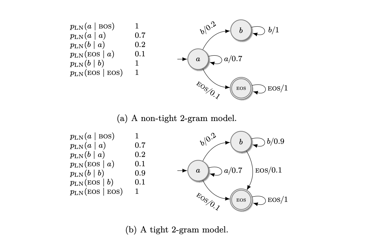
In the example (a) this happens since the only sequences that end with EOS are those that don’t produce $b$ (description of non-tight 2-gram model where sum = 1/3 <1).
It is related to the fact that the probability of EOS is 0 for some sequences, but making $p(\mathrm{EOS} \mid y_{<i}) > 0$ isn’t sufficient nor necessary.

Defining the Probability Measure of an LNM

We want to investigate what $p_\mathrm{LN}$ is when it is not an LM.
We have to be careful since the set of infinite sequences is uncountable.
We can define them as probability measures over the union of the set of finite and infinite sequences.
Definition: Sequence model is a probability space over $\Sigma^* \cup \Sigma^\infty$.
Definition: Language model is a sequence model over $\Sigma^*$ or an SM which $\mathbb{P}(\Sigma^\infty) = 0$.

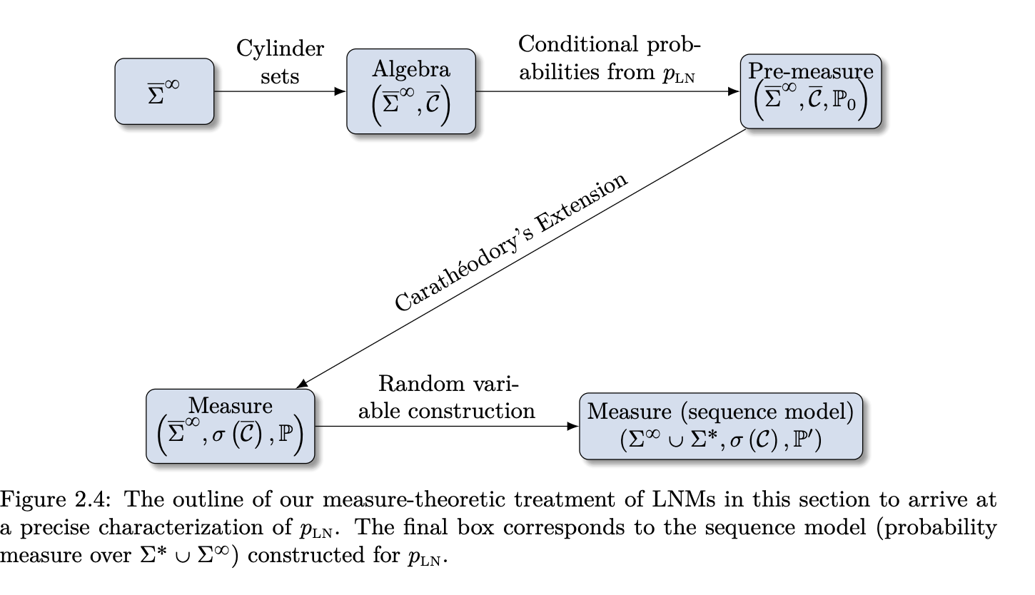
Defining an Algebra over $\bar{\Sigma}^\infty$ (Step 1)

An LNM produces conditionals over the augmented alphabet $\bar{\Sigma}$.
We will construct a sigma-algebra over $\bar{\Sigma}^\infty$ (includes both finite and infinite sequences with EOS multiple times).
Then, based on $p_\mathrm{LN}$, we will find its pre-measure that is consistent with $p_\mathrm{LN}$.
Definition: Cylinder set of rank $k$, set of infinite strings that share their $k$-prefix where $\mathcal{H} \subseteq \bar{\Sigma}^k$. \[\bar{C}(\mathcal{H}) \stackrel{\mathrm{def}}{=} \{\mathbf{y} \boldsymbol{\omega} : \mathbf{y} \in \mathcal{H}, \boldsymbol{\omega} \in \bar{\Sigma}^\infty\}.\]
Collection of all rank $k$ cylinder sets is denoted as $\mathcal{C}_k = \{\bar{C}(\mathcal{H}) \mid \mathcal{H} \in \mathcal{P}(\bar{\Sigma}^k)\}$.
This is a set of sets, so the elements of this set are cylinder sets.
This sequence is increasing, so $\mathcal{C}_1 \subseteq \mathcal{C}_2 \subseteq \ldots$.
Definition: The collection of all cylinder sets on $\Omega$ is $\mathcal{C} = \bigcup_{k=1}^{\infty} \mathcal{C}_k$.
This is an algebra over $\bar{\Sigma}^\infty$.

Defining a Pre-measure (Step 2)

We are constructing a pre-measure $\mathbb{P}_0$ for the cylinder set $\bar{C}$ given an LNM $p_\mathrm{LN}$, and any cylinder $\bar{C}(\mathcal{H}) \in \mathcal{C}$. \[\mathbb{P}_0(\bar{C}(\mathcal{H})) \stackrel{\mathrm{def}}{=} \sum_{\bar{\mathbf{y}} \in \mathcal{H}} p_\mathrm{LN}(\bar{\mathbf{y}}).\]
We measure this cylinder by summing over all the finite sequences that generate it.
Where $p_\mathrm{LN}(\bar{\mathbf{y}}) = \prod_{i=1}^{T} p_\mathrm{LN}(\bar{y}_i \mid \bar{\mathbf{y}}_{<i})$.
The same cylinder set can have different generator sets, so we have to prove that the function will have the same value for all of them.
The proofs are skipped; this is just an outline.

Extending Pre-measure into a Measure (Step 3)

For this, we will use the Carathéodory extension theorem.
Theorem: Given an algebra $\mathcal{A}$ over a set $\Omega$, if $\mathbb{P}_0$ is a pre-measure on $\mathcal{A}$, then there exists a probability space $(\Omega, \mathcal{F}, \mathbb{P})$ such that $\mathcal{A} \subseteq \mathcal{F}$ and $\mathbb{P}|_{\mathcal{A}} = \mathbb{P}_0$. Furthermore, the sigma-algebra $\mathcal{F}$ depends only on $\mathcal{A}$ and is minimal and unique, which we denote $\sigma(\mathcal{A})$, and the probability measure is unique.
Using this, we get the space $(\bar{\Sigma}^\infty, \sigma(\mathcal{C}), \mathbb{P})$.

Defining a Sequence Model (Step 4)

We have created this measure on the extended alphabet, which allows us to measure sequences that contain EOS multiple times.
We can define a random variable (RV) to map into EOS-free sequences.
RV is a measurable function between two sigma-algebras.
We want to map to outcome space $\Sigma^\infty \cup \Sigma^*$.
We can do this in the same way as before using cylinder sets where we use prefixes from $\Sigma^*$. \[C(\mathcal{H}) \stackrel{\mathrm{def}}{=} \{\mathbf{y} \boldsymbol{\omega} : \mathbf{y} \in \mathcal{H}, \boldsymbol{\omega} \in \Sigma^* \cup \Sigma^{\infty}\}.\]
Notice that now the elements of the cylinder can be also finite.
We can define the RV \[\mathrm{x}: (\bar{\Sigma}^{\infty}, \sigma(\bar{\mathcal{C}})) \rightarrow (\Sigma^* \cup \Sigma^{\infty}, \sigma(\mathcal{C})),\] which is a measurable mapping \[\mathrm{x}(\boldsymbol{\omega})= \begin{cases} \boldsymbol{\omega}_{<k} & \text{if $k$ is the first EOS in $\boldsymbol{\omega}$}, \\ \boldsymbol{\omega} & \text{otherwise (if EOS $\notin \boldsymbol{\omega}$)}. \end{cases}\]
So this mapping takes an infinite sequence containing EOS and cuts it before the first occurrence, or returns the whole sequence if EOS is not present.
So this defines a probability space $(\Sigma^* \cup \Sigma^\infty, \sigma(\mathcal{C}), \mathbb{P}_*)$.
We have done it!! Given any LNM, we can construct an associated SM, a probability space over $\Sigma^* \cup \Sigma^\infty$ where probabilities assigned to finite sequences are the same as in the LNM.

Interpreting the Constructed Probability Space

For finite $\mathbf{y} \in \Sigma^*$, $\mathbb{P}_*(\mathbf{y}) = p_\mathrm{LN}(\mathrm{EOS} \mid \mathbf{y}) p_\mathrm{LN}(\mathbf{y})$.
$\mathbb{P}_*(\Sigma^\infty)$ is the probability of generating an infinite string.
Singletons $\{\mathbf{y}\}$ and $\Sigma^\infty$ are measurable.
Proposition: A sequence model is tight iff $\sum_{\mathbf{y} \in \Sigma^*} \mathbb{P}_*(\{\mathbf{y}\}) = 1$.
EOS probability emerges as conditional probability of exact string given prefix.

\[ \begin{aligned} p_{\mathrm{LN}}(\mathrm{EOS} \mid \boldsymbol{y}) & =\frac{\mathbb{P}_*(\mathrm{x}=\boldsymbol{y})}{p_{\mathrm{LN}}(\boldsymbol{y})} \\ & =\frac{\mathbb{P}_*(\mathrm{x}=\boldsymbol{y})}{\mathbb{P}_*(\mathrm{x} \in \mathcal{C}(\boldsymbol{y}))} \\ & =\mathbb{P}_*(\mathrm{x}=\boldsymbol{y} \mid \mathrm{x} \in \mathcal{C}(\boldsymbol{y})) \end{aligned} \]

Characterizing Tightness

Event $A_k = \{\boldsymbol{\omega} \in \bar{\Sigma}^\infty : \omega_k = \mathrm{EOS}\}$.
Infinite strings: $\bigcap_{k=1}^\infty A_k^c$.
Tight if $\mathbb{P}(\bigcap_{k=1}^\infty A_k^c) = 0$.
Define $\tilde{p}_\mathrm{EOS}(t) = \mathbb{P}(A_t \mid \bigcap_{m=1}^{t-1} A_m^c) = \frac{\sum_{\boldsymbol{\omega} \in \Sigma^{t-1}} p_\mathrm{LN}(\boldsymbol{\omega}) p_\mathrm{LN}(\mathrm{EOS} \mid \boldsymbol{\omega})}{\sum_{\boldsymbol{\omega} \in \Sigma^{t-1}} p_\mathrm{LN}(\boldsymbol{\omega})}$.
Theorem (sufficient and necessary condition for tightness): An LNM is tight iff $\tilde{p}_\mathrm{EOS}(t) = 1$ for some $t$ or $\sum_{t=1}^\infty \tilde{p}_\mathrm{EOS}(t) = \infty$.
- Proof: Uses product of conditionals equaling intersection probability; applies Corollary from Borel-Cantelli for series divergence.
Borel-Cantelli Lemmas:
- I: If $\sum \mathbb{P}(A_n) < \infty$, then $\mathbb{P}(A_n$ i.o.) = 0.
- II: If independent and $\sum \mathbb{P}(A_n) = \infty$, then $\mathbb{P}(A_n$ i.o.) = 1.
- where i.o. means infinitely often which is the same as $\bigcap_{n=1}^\infty \bigcup_{k=n}^\infty A_k$.
Corollary: $\prod_{n=1}^\infty (1 - p_n) = 0 \iff \sum_{n=1}^\infty p_n = \infty$.
Theorem (sufficient condition for tightness): If $p_\mathrm{LN}(\mathrm{EOS} \mid \mathbf{y}) \geq f(t)$ for all $\mathbf{y} \in \Sigma^t$ and $\sum_{t=1}^\infty f(t) = \infty$, then tight.
Lower bound via conditional probabilities summing to infinity implies zero mass on infinite intersection. In other words, if the probability of EOS given a prefix is bounded from below by a function that diverges, then the model is tight.
$\tilde{p}_\mathrm{EOS}(t)$ often intractable due to partition function and therefore the lower bound is used in practice.