Measure Theory Recap

It is not trivial to define a language model over an uncountable set of sequences.
We need some measure-theoretic tools to avoid paradoxes.
Most technical papers aren’t rigorous enough and assume things will work out.
$\Omega$ is the sample space (event space), $\mathcal{F}$ is the sigma-algebra (measurable sets), $\mathbb{P}$ is the probability measure.
A probability space is a triple $(\Omega, \mathcal{F}, \mathbb{P})$ where:
- Definition: Sigma-algebra. $\mathcal{F} \subseteq 2^\Omega$ is a sigma-algebra if:
  - $\emptyset \in \mathcal{F}$.
  - $A \in \mathcal{F} \implies A^c \in \mathcal{F}$.
  - $A_1, A_2, \ldots$ is a countable collection in $\mathcal{F} \implies \bigcup_{i=1}^\infty A_i \in \mathcal{F}$.
- Examples: The trivial sigma-algebra $\{\emptyset, \Omega\}$ or the whole power set (discrete sigma-algebra).
Definition: Probability measure over a measurable space $(\Omega, \mathcal{F})$ is a function $\mathbb{P}: \mathcal{F} \to [0, 1]$ such that:
- $\mathbb{P}(\Omega) = 1$.
- If $A_1, A_2, \ldots$ are countable disjoint sets in $\mathcal{F}$, then $\mathbb{P}(\bigcup_{i=1}^\infty A_i) = \sum_{i=1}^\infty \mathbb{P}(A_i)$, which is called sigma-additivity.
We usually cannot have $\mathcal{F} = 2^\Omega$ because then it is provably impossible to define a probability measure that would have desired properties.
Definition: Algebra. Like a sigma-algebra but only with finite unions.
Definition: Probability pre-measure. Like a probability measure but the sigma-additivity has to hold only for unions that are in the algebra (since it’s defined over an algebra).
Carathéodory’s extension theorem: Allows us to construct simply an algebra over the set with a pre-measure and then extend it to a sigma-algebra while making this extension minimal and unique.
Definition: Random variable. A function $X: \Omega \to \mathbb{R}$ between two measurable spaces $(\Omega, \mathcal{F})$ and $(\mathbb{R}, \mathcal{B})$ (Borel sigma-algebra) is a random variable or a measurable mapping if for all sets $B \in \mathcal{B}$, we have $X^{-1}(B) \in \mathcal{F}$.
Each random variable defines a new pushforward probability measure $\mathbb{P}_X$ on $(\mathbb{R}, \mathcal{B})$ such that $\mathbb{P}_X(B) = \mathbb{P}(X^{-1}(B))$ for all $B \in \mathcal{B}$.

Language Models: Distributions over Strings

Inspiration from formal language theory which works with sets of structures, the simplest of which is a string.
Alphabet: Finite non-empty set of symbols $\Sigma$.
A string over an alphabet $\Sigma$ is a finite sequence of symbols from $\Sigma$, denoted as $s = s_1 s_2 \ldots s_n$ where $s_i \in \Sigma$.
A string can be called a word.
$|s|$ is the length of the string.
Only one string of length 0, the empty string $\epsilon$.
New strings are formed by concatenation, e.g., $s_1 s_2$ is a string of length $|s_1| + |s_2|$, which is an associative operation.
Concatenation with $\epsilon$ is the identity operation, aka $\epsilon$ is the unit and the operation is monoidal.
Kleene star: $\Sigma^* = \bigcup_{n=0}^\infty \Sigma^n$ where $\Sigma^n = \Sigma \times \Sigma \times \ldots \times \Sigma$ ($n$ times).
We also define $\Sigma^+ = \bigcup_{n=1}^\infty \Sigma^n$, which is the set of all non-empty strings over $\Sigma$.
We also define the set of all infinite strings over $\Sigma$ as $\Sigma^\infty = \Sigma \times \Sigma \times \ldots$ (infinitely many times).
In computer science (CS), strings are usually finite (not everywhere).
Kleene star contains all finite strings, including the empty string, and is countably infinite.
The set of infinite strings is uncountable for alphabets with more than one symbol.
Definition: Language. Let $\Sigma$ be an alphabet, then a language over $\Sigma$ is a subset of $\Sigma^*$.
If not specified, we usually assume the language is the whole Kleene star.
Subsequence: A string $s$ is a subsequence of a string $t$ if we can obtain $s$ by deleting some symbols from $t$ without changing the order of the remaining symbols.
Substring: A contiguous subsequence.
Prefix and suffix are special cases of substrings that share the start or end of the string.
Prefix notation: $y_{<n}$ is a prefix of length $n-1$ of a string $y$.
$y \triangleleft y'$ to denote that $y$ is a suffix of $y'$.

Definition of a Language Model

Now we can write the definition of a language model.
Definition: $\Sigma$ is an alphabet, then a language model is a discrete distribution $p_\mathrm{LM}$ over $\Sigma^*$.
Definition: Weighted language is $L(p_\mathrm{LM}) = \{(s, p_\mathrm{LM}(s)) \mid s \in \Sigma^* \}$.
We haven’t yet said how to represent such a distribution.

Global and Local Normalization

By definition, a language model is always tight.
So by non-tight language models that appear often in practice, we mean that the distribution is not normalized, so it’s technically not a language model, and “tight” acts as a non-intersective adjective.
These non-tight models do appear, for example, from recurrent neural networks (RNNs) trained from data.
Depending on whether we model the probability of the whole string or the next symbol, we can have global or local normalization.
BOS token is a special token that indicates the start of a sequence, so it’s gonna be $y_0$.
Augmented alphabet: $\bar{\Sigma} = \Sigma \cup \{\mathrm{EOS}\}$.
And also Kleene star of this set is $\bar{\Sigma}^*$.
Models that are leaking probability mass to infinite sequences will be called sequence models.

Globally Normalized Language Model or Energy Model

Definition: Energy function $\hat{p}: \Sigma^* \to \mathbb{R}$.
Inspired from statistical physics, an energy function can be used to define a probability distribution by exponentiating its negative value.
Definition: Globally normalized language model is a function $p_\mathrm{LM}: \Sigma^* \to [0, 1]$ such that: \[p_\mathrm{LM}(s) = \frac{e^{-\hat{p}(s)}}{\sum_{s' \in \Sigma^*} e^{-\hat{p}(s')}}.\]
They are easy to define, but hard to compute the normalization constant.
Definition: Normalizable energy function has a finite normalizer; if not, then it’s ill-defined.
Any normalizable energy function induces a language model over $\Sigma^*$.
In general, it’s undecidable if it’s normalizable; even if so, it can be computationally impossible; it’s also hard to sample from the distribution.

Locally Normalized Models

We have to know when the termination ends: $\bar{\Sigma} = \Sigma \cup \{\mathrm{EOS}\}$.
Definition: (Locally normalized) sequence model is a function $p_\mathrm{SM}$ over an alphabet $\Sigma$ is a set of conditional probabilities.
$p_\mathrm{SM}(y \mid \mathbf{y})$ where $\mathbf{y} \in \Sigma^*$ is the history.
SM can be also over $\bar{\Sigma}$.
Definition: Locally normalized language model is a sequence model over $\bar{\Sigma}$ such that: \[p_\mathrm{LM}(\mathbf{y}) = p_\mathrm{SM}(\mathrm{EOS} \mid \mathbf{y}) \prod_{i=1}^{T} p_\mathrm{SM}(y_i \mid y_{<i}),\] for all $\mathbf{y} \in \Sigma^*$, with $|\mathbf{y}| = T$.
The model is tight if $1 = \sum_{\mathbf{y} \in \Sigma^*} p_\mathrm{LM}(\mathbf{y})$.
So again, an LN LM isn’t necessarily an LM; it’s about how we can write it.
When can an LM be locally normalized?
Answer: Every model can be locally normalized.
Definition: Prefix probability. $\pi(\mathbf{y}) = \sum_{\mathbf{y}' \in \Sigma^*} p_\mathrm{LM}(\mathbf{y} \mathbf{y}')$.
Probability that $\mathbf{y}$ is a prefix of any string in the language, the cumulative probability of all strings that start with that prefix.
Theorem: Let $p_\mathrm{LM}$ be a language model, then there exists an LN model such that for all $\mathbf{y} \in \Sigma^*$, $p_\mathrm{LM} = p_\mathrm{LN}(\mathbf{y}) = p_\mathrm{SM}(\mathrm{EOS} \mid \mathbf{y}) \prod_{i=1}^{T} p_\mathrm{SM}(y_i \mid y_{<i})$.
Sketch of proof: We define $p_\mathrm{SM}(y \mid \mathbf{y}) = \frac{\pi(\mathbf{y} y)}{\pi(\mathbf{y})}$ and $p_\mathrm{SM}(\mathrm{EOS} \mid \mathbf{y}) = \frac{p_\mathrm{LM}(\mathbf{y})}{\pi(\mathbf{y})}$.
When we then write $p_\mathrm{LN}(\mathbf{y})$ for $\pi(\mathbf{y}) > 0$, we get that it is the same as $p_\mathrm{LM}$.
And for $\pi(\mathbf{y}) = 0$, we have $p_\mathrm{LN}(\mathbf{y}) = 0$, so it’s well-defined.
LNMs are very common in natural language processing (NLP) even though they are not necessarily language models.

Tight Language Models

Locally normalized language models can be non-tight, leaking probability mass to infinite sequences.
The sum over all sequences of the LN model may not sum to one, but each conditional of $p_\mathrm{SM}$ is normalized.
Tight is sometimes called consistent or proper.

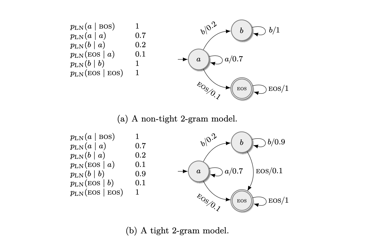
In the example (a) this happens since the only sequences that end with EOS are those that don’t produce $b$ (description of non-tight 2-gram model where sum = 1/3 <1).
It is related to the fact that the probability of EOS is 0 for some sequences, but making $p(\mathrm{EOS} \mid y_{<i}) > 0$ isn’t sufficient nor necessary.

Defining the Probability Measure of an LNM

We want to investigate what $p_\mathrm{LN}$ is when it is not an LM.
We have to be careful since the set of infinite sequences is uncountable.
We can define them as probability measures over the union of the set of finite and infinite sequences.
Definition: Sequence model is a probability space over $\Sigma^* \cup \Sigma^\infty$.
Definition: Language model is a sequence model over $\Sigma^*$ or an SM which $\mathbb{P}(\Sigma^\infty) = 0$.

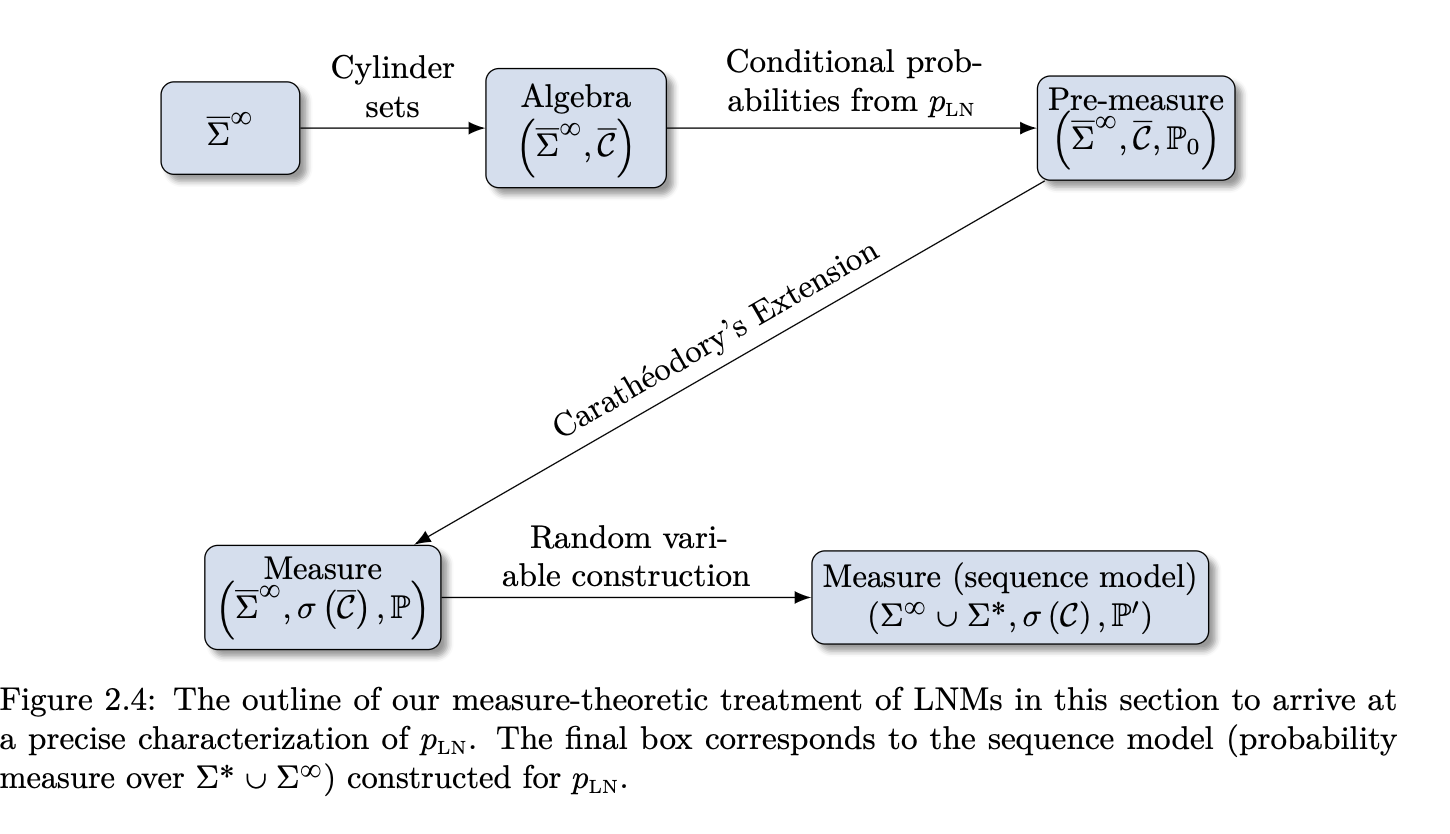
Defining an Algebra over $\bar{\Sigma}^\infty$ (Step 1)

An LNM produces conditionals over the augmented alphabet $\bar{\Sigma}$.
We will construct a sigma-algebra over $\bar{\Sigma}^\infty$ (includes both finite and infinite sequences with EOS multiple times).
Then, based on $p_\mathrm{LN}$, we will find its pre-measure that is consistent with $p_\mathrm{LN}$.
Definition: Cylinder set of rank $k$, set of infinite strings that share their $k$-prefix where $\mathcal{H} \subseteq \bar{\Sigma}^k$. \[\bar{C}(\mathcal{H}) \stackrel{\mathrm{def}}{=} \{\mathbf{y} \boldsymbol{\omega} : \mathbf{y} \in \mathcal{H}, \boldsymbol{\omega} \in \bar{\Sigma}^\infty\}.\]
Collection of all rank $k$ cylinder sets is denoted as $\mathcal{C}_k = \{\bar{C}(\mathcal{H}) \mid \mathcal{H} \in \mathcal{P}(\bar{\Sigma}^k)\}$.
This is a set of sets, so the elements of this set are cylinder sets.
This sequence is increasing, so $\mathcal{C}_1 \subseteq \mathcal{C}_2 \subseteq \ldots$.
Definition: The collection of all cylinder sets on $\Omega$ is $\mathcal{C} = \bigcup_{k=1}^{\infty} \mathcal{C}_k$.
This is an algebra over $\bar{\Sigma}^\infty$.

Defining a Pre-measure (Step 2)

We are constructing a pre-measure $\mathbb{P}_0$ for the cylinder set $\bar{C}$ given an LNM $p_\mathrm{LN}$, and any cylinder $\bar{C}(\mathcal{H}) \in \mathcal{C}$. \[\mathbb{P}_0(\bar{C}(\mathcal{H})) \stackrel{\mathrm{def}}{=} \sum_{\bar{\mathbf{y}} \in \mathcal{H}} p_\mathrm{LN}(\bar{\mathbf{y}}).\]
We measure this cylinder by summing over all the finite sequences that generate it.
Where $p_\mathrm{LN}(\bar{\mathbf{y}}) = \prod_{i=1}^{T} p_\mathrm{LN}(\bar{y}_i \mid \bar{\mathbf{y}}_{<i})$.
The same cylinder set can have different generator sets, so we have to prove that the function will have the same value for all of them.
The proofs are skipped; this is just an outline.

Extending Pre-measure into a Measure (Step 3)

For this, we will use the Carathéodory extension theorem.
Theorem: Given an algebra $\mathcal{A}$ over a set $\Omega$, if $\mathbb{P}_0$ is a pre-measure on $\mathcal{A}$, then there exists a probability space $(\Omega, \mathcal{F}, \mathbb{P})$ such that $\mathcal{A} \subseteq \mathcal{F}$ and $\mathbb{P}|_{\mathcal{A}} = \mathbb{P}_0$. Furthermore, the sigma-algebra $\mathcal{F}$ depends only on $\mathcal{A}$ and is minimal and unique, which we denote $\sigma(\mathcal{A})$, and the probability measure is unique.
Using this, we get the space $(\bar{\Sigma}^\infty, \sigma(\mathcal{C}), \mathbb{P})$.

Defining a Sequence Model (Step 4)

We have created this measure on the extended alphabet, which allows us to measure sequences that contain EOS multiple times.
We can define a random variable (RV) to map into EOS-free sequences.
RV is a measurable function between two sigma-algebras.
We want to map to outcome space $\Sigma^\infty \cup \Sigma^*$.
We can do this in the same way as before using cylinder sets where we use prefixes from $\Sigma^*$. \[C(\mathcal{H}) \stackrel{\mathrm{def}}{=} \{\mathbf{y} \boldsymbol{\omega} : \mathbf{y} \in \mathcal{H}, \boldsymbol{\omega} \in \Sigma^* \cup \Sigma^{\infty}\}.\]
Notice that now the elements of the cylinder can be also finite.
We can define the RV \[\mathrm{x}: (\bar{\Sigma}^{\infty}, \sigma(\bar{\mathcal{C}})) \rightarrow (\Sigma^* \cup \Sigma^{\infty}, \sigma(\mathcal{C})),\] which is a measurable mapping \[\mathrm{x}(\boldsymbol{\omega})= \begin{cases} \boldsymbol{\omega}_{<k} & \text{if $k$ is the first EOS in $\boldsymbol{\omega}$}, \\ \boldsymbol{\omega} & \text{otherwise (if EOS $\notin \boldsymbol{\omega}$)}. \end{cases}\]
So this mapping takes an infinite sequence containing EOS and cuts it before the first occurrence, or returns the whole sequence if EOS is not present.
So this defines a probability space $(\Sigma^* \cup \Sigma^\infty, \sigma(\mathcal{C}), \mathbb{P}_*)$.
We have done it!! Given any LNM, we can construct an associated SM, a probability space over $\Sigma^* \cup \Sigma^\infty$ where probabilities assigned to finite sequences are the same as in the LNM.

Interpreting the Constructed Probability Space

For finite $\mathbf{y} \in \Sigma^*$, $\mathbb{P}_*(\mathbf{y}) = p_\mathrm{LN}(\mathrm{EOS} \mid \mathbf{y}) p_\mathrm{LN}(\mathbf{y})$.
$\mathbb{P}_*(\Sigma^\infty)$ is the probability of generating an infinite string.
Singletons $\{\mathbf{y}\}$ and $\Sigma^\infty$ are measurable.
Proposition: A sequence model is tight iff $\sum_{\mathbf{y} \in \Sigma^*} \mathbb{P}_*(\{\mathbf{y}\}) = 1$.
EOS probability emerges as conditional probability of exact string given prefix.

\[ \begin{aligned} p_{\mathrm{LN}}(\mathrm{EOS} \mid \boldsymbol{y}) & =\frac{\mathbb{P}_*(\mathrm{x}=\boldsymbol{y})}{p_{\mathrm{LN}}(\boldsymbol{y})} \\ & =\frac{\mathbb{P}_*(\mathrm{x}=\boldsymbol{y})}{\mathbb{P}_*(\mathrm{x} \in \mathcal{C}(\boldsymbol{y}))} \\ & =\mathbb{P}_*(\mathrm{x}=\boldsymbol{y} \mid \mathrm{x} \in \mathcal{C}(\boldsymbol{y})) \end{aligned} \]

Characterizing Tightness

Event $A_k = \{\boldsymbol{\omega} \in \bar{\Sigma}^\infty : \omega_k = \mathrm{EOS}\}$.
Infinite strings: $\bigcap_{k=1}^\infty A_k^c$.
Tight if $\mathbb{P}(\bigcap_{k=1}^\infty A_k^c) = 0$.
Define $\tilde{p}_\mathrm{EOS}(t) = \mathbb{P}(A_t \mid \bigcap_{m=1}^{t-1} A_m^c) = \frac{\sum_{\boldsymbol{\omega} \in \Sigma^{t-1}} p_\mathrm{LN}(\boldsymbol{\omega}) p_\mathrm{LN}(\mathrm{EOS} \mid \boldsymbol{\omega})}{\sum_{\boldsymbol{\omega} \in \Sigma^{t-1}} p_\mathrm{LN}(\boldsymbol{\omega})}$.
Theorem (sufficient and necessary condition for tightness): An LNM is tight iff $\tilde{p}_\mathrm{EOS}(t) = 1$ for some $t$ or $\sum_{t=1}^\infty \tilde{p}_\mathrm{EOS}(t) = \infty$.
- Proof: Uses product of conditionals equaling intersection probability; applies Corollary from Borel-Cantelli for series divergence.
Borel-Cantelli Lemmas:
- I: If $\sum \mathbb{P}(A_n) < \infty$, then $\mathbb{P}(A_n$ i.o.) = 0.
- II: If independent and $\sum \mathbb{P}(A_n) = \infty$, then $\mathbb{P}(A_n$ i.o.) = 1.
- where i.o. means infinitely often which is the same as $\bigcap_{n=1}^\infty \bigcup_{k=n}^\infty A_k$.
Corollary: $\prod_{n=1}^\infty (1 - p_n) = 0 \iff \sum_{n=1}^\infty p_n = \infty$.
Theorem (sufficient condition for tightness): If $p_\mathrm{LN}(\mathrm{EOS} \mid \mathbf{y}) \geq f(t)$ for all $\mathbf{y} \in \Sigma^t$ and $\sum_{t=1}^\infty f(t) = \infty$, then tight.
Lower bound via conditional probabilities summing to infinity implies zero mass on infinite intersection. In other words, if the probability of EOS given a prefix is bounded from below by a function that diverges, then the model is tight.
$\tilde{p}_\mathrm{EOS}(t)$ often intractable due to partition function and therefore the lower bound is used in practice.

Modeling Foundations

The decisions when we want to build a distribution over strings and estimate its parameters.
How can a sequence model be parameterized?
$p_{\omega}: \Sigma^* \rightarrow \mathbb{R}$, where $\Sigma^*$ denotes the Kleene closure of the alphabet $\Sigma$.
Where parameters $\omega \in \Theta$ are free parameters of the function.
Given a parameterized model, how can the parameters be chosen to best reflect the data?

Representation-Based Language Models

Most modern language models are defined as locally normalized (LN) models.
However, we first define a sequence model and prove that a specific parameterization encodes a tight LN model.
We parameterize to enable optimization with respect to some objective.
One way is to embed individual symbols and possible contexts into a Hilbert space, enabling a notion of similarity.
Principle: Good representation principle: The success of a machine learning (ML) task depends on chosen representations; in our case, representations of symbols and contexts.
Definition: Vector space over a field $\mathbb{F}$: A set $V$ with two operations—addition and scalar multiplication—satisfying 8 axioms (associativity, commutativity, identity element of addition, inverse elements of addition, compatibility of scalar multiplication with field multiplication, identity element of scalar multiplication, distributivity of scalar multiplication with respect to vector addition, and distributivity of scalar multiplication with respect to field addition).
A $D$-dimensional vector space has $D$ basis vectors, representable as a $D$-dimensional vector in $\mathbb{F}^D$.
An inner product is defined as a bilinear form $\langle \cdot, \cdot \rangle: V \times V \rightarrow \mathbb{F}$ satisfying (conjugate) symmetry, linearity in the first argument, and positive-definiteness.
The inner product induces a norm $\|\cdot\|: V \rightarrow \mathbb{R}_{\geq 0}$ defined as $\|v\| = \sqrt{\langle v, v \rangle}$.
Hilbert space is a complete inner product space, meaning every Cauchy sequence (or every absolutely convergent sequence in the norm) converges to a limit in the space.
An inner product space can be completed into a Hilbert space.
We need a Hilbert space because infinite sequences (e.g., generated by a recurrent neural network, RNN) must lie in the space; e.g., using rationals as the field would not represent all sequences (limit might be irrational like $\sqrt{2}$).
Representation function from a set $\mathcal{S}$ to a Hilbert space $V$ is a function mapping elements to their representations.
If $\mathcal{S}$ is finite, it can be represented as a matrix $E \in \mathbb{R}^{|\mathcal{S}| \times D}$, where each row is the representation of a symbol.
This is the case for embedding symbols from the extended alphabet $\bar{\Sigma} = \Sigma \cup \{\mathrm{bos}, \mathrm{eos}\}$ via an embedding function $e: \bar{\Sigma} \rightarrow \mathbb{R}^D$.
E.g., one-hot encoding assigns each symbol its $n$th basis vector (matrix is identity-like); it’s sparse, and cosine similarity is 0 for non-identical symbols.
We want to capture semantic information.
For contexts, define an encoding function $\mathrm{enc}: \bar{\Sigma}^* \rightarrow \mathbb{R}^D$ mapping the context to a vector in the same space.
For now, treat the function as a black box.

Compatibility of Symbol and Context

$\cos(\theta) = \frac{\langle e(y), \mathrm{enc}(\boldsymbol{y}) \rangle}{\|e(y)\| \|\mathrm{enc}(\boldsymbol{y})\|}$.
Traditionally, use the inner product as the compatibility function.
For a symbol and context: $\langle e(y), \mathrm{enc}(\boldsymbol{y}) \rangle$.
All compatibilities via matrix multiplication: $E \cdot \mathrm{enc}(\boldsymbol{y})$.
Entries are often called scores or logits.
To formulate $p_{\mathrm{SM}}$, project the scores into a probability simplex.
Definition: Probability simplex $\Delta^{D-1} = \{\mathbf{x} \in \mathbb{R}^D \mid x_d \geq 0, \sum_{d=1}^D x_d = 1\}$.
$p_{\mathrm{SM}}: V \rightarrow \Delta^{|\bar{\Sigma}|-1}$.
Need a projection function from logits to the simplex.
Requires monotonicity, positivity everywhere, and summing to 1.
Definition: Softmax function:
- $\mathrm{softmax}: \mathbb{R}^D \rightarrow \Delta^{D-1}$.
- $\mathrm{softmax}(\mathbf{x})_d = \frac{\exp(x_d / \varepsilon)}{\sum_{j=1}^D \exp(x_j / \varepsilon)}$, where $\varepsilon > 0$ is the temperature.
Temperature $\varepsilon$ controls entropy by scaling logits; in the Boltzmann distribution context, it relates to randomness.
High $\varepsilon$: More uniform distribution; low $\varepsilon$: More peaked; limit as $\varepsilon \to 0^+$: Argmax (one-hot at maximum).
Variational characterization: \[ \mathrm{softmax}(\mathbf{x}) = \underset{\mathbf{p} \in \Delta^{D-1}}{\mathrm{argmax}} \left( \mathbf{p}^\top \mathbf{x} - \varepsilon \sum_{d=1}^D p_d \log p_d \right) = \underset{\mathbf{p} \in \Delta^{D-1}}{\mathrm{argmax}} \left( \mathbf{p}^\top \mathbf{x} + \varepsilon H(\mathbf{p}) \right), \] where $H(\mathbf{p}) = -\sum_d p_d \log p_d$ is entropy.
Interpreted as the vector with maximal similarity to $\mathbf{x}$ while regularized for high entropy.
Non-sparse (zeros only if input is $-\infty$).
Invariant to constant addition: $\mathrm{softmax}(\mathbf{x} + c \mathbf{1}) = \mathrm{softmax}(\mathbf{x})$.
Derivative is computable and function is smooth.
Maintains ordering for all temperatures: If $x_i > x_j$, then $\mathrm{softmax}(\mathbf{x})_i > \mathrm{softmax}(\mathbf{x})_j$.
Other projections like sparsemax: $\mathrm{sparsemax}(\mathbf{x}) = \underset{\mathbf{p} \in \Delta^{D-1}}{\mathrm{argmin}} \|\mathbf{p} - \mathbf{x}\|_2^2$ (can be sparse, but not everywhere differentiable).

Representation-Based Locally Normalized Language Model

Definition: \[ p_{\mathrm{SM}}(y_t \mid \boldsymbol{y}_{<t}) \stackrel{\text{def}}{=} f_{\Delta^{|\bar{\Sigma}|-1}} \left( E \cdot \mathrm{enc}(\boldsymbol{y}_{<t}) \right)_{y_t}, \] where $f$ is typically softmax.
Defines probability of whole string: $p_{\mathrm{LN}}(\boldsymbol{y}) = p_{\mathrm{SM}}(\mathrm{eos} \mid \boldsymbol{y}) \prod_{t=1}^T p_{\mathrm{SM}}(y_t \mid \boldsymbol{y}_{<t})$, with $\boldsymbol{y}_0 = \mathrm{bos}$.
Encoding functions carry all information about symbol likelihoods given contexts.
Theorem: Let $p_{\mathrm{SM}}$ be a representation-based sequence model over alphabet $\Sigma$.
- $s \stackrel{\text{def}}{=} \sup_{y \in \Sigma} \|e(y) - e(\mathrm{eos})\|_2$ (largest distance to eos representation).
- $z_{\max}^t = \max_{\boldsymbol{y} \in \Sigma^t} \|\mathrm{enc}(\boldsymbol{y})\|_2$ (maximum context norm for length $t$).
- LN model induced by $p_{\mathrm{SM}}$ is tight if $s z_{\max}^t \leq \log t$.
Theorem: Representation-based LN models with uniformly bounded $\|\mathrm{enc}(\boldsymbol{y})\|_p$ for some $p \geq 1$ are tight.
Often holds in practice due to bounded activation functions, ensuring softmax assigns positive probability to eos.

Estimating a Language Model

$D$ is a collection of $N$ i.i.d. strings from $\Sigma^*$ generated according to the unknown $p_{\mathrm{LM}}$ distribution.
This is often posed as an optimization problem or search for the best parameters; therefore, we must limit the space of possible models.
We limit ourselves to a parameterized family of models $\{p_{\omega} \mid \omega \in \Theta\}$, where $\Theta$ is the parameter space.
General Framework
- We search for parameters $\hat{\omega}$ that maximize a chosen objective, or alternatively, minimize some loss function $\varsigma: \Theta \times \Theta \rightarrow \mathbb{R}_{\geq 0}$.
- We seek the model $\hat{\omega} = \arg\min_{\omega \in \Theta} \varsigma(\omega^*, \omega)$.
- We don’t know $\omega^*$ but can estimate it using the empirical distribution from the corpus pointwise.
- Definition: $\hat{p}_{\omega^*}(\boldsymbol{y}) = \frac{1}{N} \sum_{n=1}^N \delta_{\boldsymbol{y}^{(n)}}(\boldsymbol{y})$.
- This can also be decomposed on the level of the symbols.
- We focus on the generative paradigm where we model the distribution not just boundaries between classes; this is usually the case for language models where we use unannotated data with self-supervised learning.
- We can now measure the distance between these distributions using cross-entropy, which has its roots in information theory.
- $\varsigma(\omega^*, \omega) = H(\hat{p}_{\omega^*}, p_{\omega})$.
- In general, cross-entropy is defined as $H(p_1, p_2) = -\sum_{\boldsymbol{y} \in \mathcal{Y}} p_1(\boldsymbol{y}) \log p_2(\boldsymbol{y})$, where the sum is over the support $\mathcal{Y}$ of $p_1$.
- Usually written in the LN form: $H(p_1, p_2) = -\sum_{\boldsymbol{y} \in \mathcal{Y}} \sum_{t=1}^T p_1(y_t \mid \boldsymbol{y}_{<t}) \log p_2(y_t \mid \boldsymbol{y}_{<t})$.
- CE is not symmetric; CE between two distributions is the average number of bits needed to encode samples from $p_1$ using a code optimized for $p_2$.
- The optimal encoding for $p_1$ uses $-\log p_1(y)$ bits to encode an event with prob $p_1(y)$, so the minimal value for CE is when $p_1 = p_2$.
- Related to KL divergence, which is defined as $D_{\mathrm{KL}}(p_1 \| p_2) = H(p_1, p_2) - H(p_1, p_1)$, which could be used as a loss with the same results since the entropy term doesn’t depend on the parameters.
Relationship to MLE
- Data likelihood $\mathcal{L}(\omega) = \prod_{n=1}^N p_{\omega}(\boldsymbol{y}^{(n)})$.
- Principle: The optimal parameters are those that maximize the likelihood of the data observed.
- We usually work with log-likelihood, since it’s convex and numerically more stable.
- The optimal parameters found using MLE are the same as those found using minimizing the cross-entropy loss with empirical distribution.
- These multiple perspectives show us that we want to be close w.r.t. a given metric and place probability mass on the observed data.
- Theorem: MLE is consistent: Consider loss $\varsigma(\omega^*, \omega) = H(\hat{p}_{\omega^*}, p_{\omega})$ and that data is i.i.d. generated from the language model. Under regularity conditions for the parametric family and that the minimizer is unique, the estimator $\hat{\omega}$ is a consistent estimator, i.e., it converges in probability as $N \rightarrow \infty$ to the true parameters $\omega^*$.
- Up to here we assumed that the optimal model lives in the parametric space, which in practice is not the case; we can still prove relationship between the true model and its projection onto the parametric space being close to the estimated model.
Problems with CE: The model has to place mass on all strings in $\Sigma^*$, to avoid infinite loss; this is called mean-seeking behavior.
It is unclear whether this is desirable or not.
Teacher forcing: We have only considered loss functions that condition on the previous symbol, like a time series, and even if the model predicts wrong, we condition in the next step on the ground truth; training with CE mandates this, but this can lead to bad performance if we score the model’s prediction on a whole sequence; this is called exposure bias. On the other hand, using previous predictions can lead to training instability.
Masked Language Modeling
- Sequential conditioning useful for generation.
- But seeing both the previous and next symbol is useful for classification.
- Sometimes called pseudo-log-likelihood. \[ \ell_{\mathrm{MLM}}(\omega)=\sum_{n=1}^N\sum_{t=1}^T\log p_\omega(y_t^{(n)}\mid\boldsymbol{y}_{<t}^{(n)},\boldsymbol{y}_{>t}^{(n)}). \]
- BERT (2019) best known masked language model.
- They are not LMs in the strict sense since they don’t model a valid distribution over $\Sigma^*$.
- Popular for language tasks and fine-tuning.
Other Divergence Measures
- There has been work on using other divergence measures that can better capture the tails of the distributions since language has long tail, in contrast to mean-seeking behavior of CE.
- There are computational issues with other measures.
- For example, we can estimate the forward KL using MC only using the samples from the data but we don’t have access to the true distribution.
Scheduled Sampling (Bengio 2015)
- After initial period, some part of predictions is conditioned on the previous prediction, rather than the ground truth.
- This is done to avoid exposure bias.
- The estimator no longer consistent.
- These and other methods aim to specify an alternative distribution of high-quality texts rather than average texts and use RL methods like the REINFORCE algorithm to optimize the model.
- There can be also other auxiliary tasks that are intertwined in the training like next sentence prediction, frequency prediction, sentence order prediction, etc.; these methods usually lead to invalidate the formal requirements for a true LM.

Parameter Estimation

Finding best parameters analytically or manually is not possible.
We have to resort to numerical optimization.
To have an unbiased estimate of the model performance we have to split the data into training, validation, and test set.
Most are gradient methods.
Backprop = reverse-mode autodiff.
We can compute gradients with the same complexity as the forward pass.
Normal GD is over the whole dataset, but this is not feasible for large datasets.
Usually we use SGD or mini-batch SGD to estimate the gradients but trade off higher variance.
Curriculum learning: Start with easy training examples and gradually increase the difficulty.
Usually ADAM that uses estimates of the first and second moments of the gradients; this is often used in practice.
Parameter initialization is very important, can result in bad local minima or slow convergence; Xavier or He for ReLU.
Early stopping: Stop training when the validation loss stops improving; this is to avoid overfitting, though recently people observe double descent or grokking which suggests learning longer may be beneficial in specific cases.
Regularization: Is a technique which modifies the training with the intention of improving generalization performance perhaps at the cost of training performance, aka making the training harder in some way.
Most common in language models:
- Weight decay: Sometimes called L2 regularization, penalizes large weights by adding a term to the loss function that is proportional to the square of the magnitude of the weights.
- Entropy regularization: Principle of maximum entropy: Best prior is the one that is least informative; label smoothing and confidence penalty add terms to the loss that penalize peaky distributions.
- Dropout: Randomly sets a fraction of the activations to zero during training; this avoids overly relying on a specific signal and also can be viewed as an ensemble method.
- Batch and layer norm:
  - Batch norm: Normalizes the activations of a layer across the batch; this helps with convergence and stability.
  - Layer norm: Normalizes the activations across the features; this is often used in transformer models.

Classical Language Models

This chapter introduces classical language modeling frameworks, focusing on finite-state language models (a generalization of n-gram models). These older approaches distill key concepts due to their simplicity and serve as baselines for modern neural architectures discussed in Chapter 5. Key questions: How can we tractably represent conditional distributions $p_{SM}(y \mid \mathbf{y})$? How can we represent hierarchical structures in language?

Finite-State Language Models

Finite-state language models generalize n-gram models and are based on finite-state automata (FSA), which distinguish a finite number of contexts when modeling conditional distributions $p_M(y \mid \mathbf{y})$.
Informal Definition: A language model $p_{LM}$ is finite-state if it defines only finitely many unique conditional distributions $p_{LM}(y \mid \mathbf{y})$.
This bounds the number of distributions to learn but is insufficient for human language; still useful as baselines and theoretical tools.

Finite-State Automata (FSA)

Definition: An FSA is a 5-tuple $(\Sigma, Q, I, F, \delta)$, where:
- $\Sigma$ is the alphabet.
- $Q$ is a finite set of states.
- $I \subseteq Q$ is the set of initial states.
- $F \subseteq Q$ is the set of final states.
- $\delta \subseteq Q \times (\Sigma \cup \{\epsilon\}) \times Q$ is a finite multiset of transitions (notation: $q_1 \xrightarrow{a} q_2$ for $(q_1, a, q_2) \in \delta$; multiset allows duplicates).
Graphically: Labeled directed multigraph; vertices = states; edges = transitions; initial states marked by incoming arrow; final states by double circle.
FSA reads input string $y \in \Sigma^*$ sequentially, transitioning per $\delta$; starts in $I$; $\epsilon$-transitions consume no input.
Non-determinism: Multiple transitions possible; take all in parallel.
Deterministic FSA: No $\epsilon$-transitions; at most one transition per $(q, a) \in Q \times \Sigma$; single initial state.
Deterministic and non-deterministic FSAs are equivalent (can convert between them).
Accepts $y$ if ends in $F$ after reading $y$.
Language: $L(\mathcal{A}) = \{ y \mid y$ recognized by $\mathcal{A} \}$.
Regular Language: $L \subseteq \Sigma^*$ is regular iff recognized by some FSA.

Weighted Finite-State Automata (WFSA)

Augment FSA with real-valued weights.
Definition: WFSA $\mathcal{A} = (\Sigma, Q, \delta, \lambda, \rho)$, where:
- $\delta \subseteq Q \times (\Sigma \cup \{\epsilon\}) \times \mathbb{R} \times Q$ (notation: $q \xrightarrow{a/w} q'$).
- $\lambda: Q \to \mathbb{R}$ (initial weights).
- $\rho: Q \to \mathbb{R}$ (final weights).
Implicit initials: $\{q \mid \lambda(q) \neq 0\}$; finals: $\{q \mid \rho(q) \neq 0\}$.
Transition Matrix: $T(a)_{ij} =$ sum of weights from $i$ to $j$ labeled $a$; $T = \sum_{a \in \Sigma} T(a)$.
Path: Sequence of consecutive transitions; $|\pi| =$ length; $p(\pi), n(\pi) =$ origin/destination; $s(\pi) =$ yield.
Path sets: $\Pi(\mathcal{A}) =$ all paths; $\Pi(\mathcal{A}, y) =$ yielding $y$; $\Pi(\mathcal{A}, q, q') =$ from $q$ to $q'$.
Path Weight: Inner $w_I(\pi) = \prod_{n=1}^N w_n$ for $\pi = q_1 \xrightarrow{a_1/w_1} q_2 \cdots q_N$; full $w(\pi) = \lambda(p(\pi)) \cdot w_I(\pi) \cdot \rho(n(\pi))$.
Accepting: $w(\pi) \neq 0$.
Stringsum: $\mathcal{A}(y) = \sum_{\pi \in \Pi(\mathcal{A}, y)} w(\pi)$.
Weighted Language: $L(\mathcal{A}) = \{(y, \mathcal{A}(y)) \mid y \in \Sigma^*\}$; weighted regular if from WFSA.
State Allsum (backward value $\beta(q)$): $Z(\mathcal{A}, q) = \sum_{\pi: p(\pi)=q} w_I(\pi) \cdot \rho(n(\pi))$.
Allsum: $Z(\mathcal{A}) = \sum_y \mathcal{A}(y) = \sum_\pi w(\pi)$; normalizable if finite.
Accessibility: $q$ accessible if non-zero path from initial; co-accessible if to final; useful if both.
Trim: Remove useless states (preserves non-zero weights).
Probabilistic WFSA (PFSA): $\sum_q \lambda(q)=1$; weights $\geq 0$; for each $q$, $\sum w + \rho(q)=1$ over outgoing and final.
Final weights replace EOS; corresponds to locally normalized models.

Finite-State Language Models (FSLM)

Definition: $p_{LM}$ finite-state if $L(p_{LM}) = L(\mathcal{A})$ for some WFSA (weighted regular language).
Path/String Prob in PFSA: Path prob = weight; string prob $p_{\mathcal{A}}(y) = \mathcal{A}(y)$ (local; may not be tight).
String Prob in WFSA: $p_{\mathcal{A}}(y) = \mathcal{A}(y) / Z(\mathcal{A})$ (global, tight if normalizable, non-negative).
Induced LM: $p_{LM^{\mathcal{A}}}(y) = p_{\mathcal{A}}(y)$.

Normalizing Finite-State Language Models

Pairwise pathsums: $M_{ij} = \sum_{\pi: i \to j} w_I(\pi)$; $Z(\mathcal{A}) = \vec{\lambda} M \vec{\rho}$.
- Proof: Group paths by origin/destination; factor $\lambda(i), \rho(j)$.
$T^d_{ij} = \sum w_I(\pi)$ over length-$d$ paths $i \to j$ (induction).
$T^* = \sum_{d=0}^\infty T^d = (I - T)^{-1}$ if converges; $M = T^*$.
Runtime $O(|Q|^3)$; Lehmann’s algorithm special case.
Converges iff spectral radius $\rho_s(T) < 1$ (eigenvalues $<1$ in magnitude).
Speed-ups: Acyclic = linear in transitions (Viterbi); sparse components combine algorithms.
Differentiable for gradient-based training.

Locally Normalizing a Globally Normalized Finite-State Language Model

Instance of weight pushing; computes state allsums, reweights transitions.
Theorem: Normalizable non-negative WFSA and tight PFSA equally expressive.
- Proof ($\Leftarrow$): Trivial (tight PFSA is WFSA with $Z=1$).
- ($\Rightarrow$): For trim $\mathcal{A}_G$, construct $\mathcal{A}_L$ with same structure; reweight initials $\lambda_L(q) = \lambda(q) Z(\mathcal{A}, q) / Z(\mathcal{A})$; finals $\rho_L(q) = \rho(q) / Z(\mathcal{A}, q)$; transitions $w_L = w \cdot Z(\mathcal{A}, q') / Z(\mathcal{A}, q)$.
- Non-negative; sum to 1 (by allsum recursion lemma).
- Path probs match: Internal allsums cancel; leaves $w(\pi)/Z(\mathcal{A})$.
Lemma (Allsum Recursion): $Z(\mathcal{A}, q) = \sum_{q \xrightarrow{a/w} q'} w \cdot Z(\mathcal{A}, q') + \rho(q)$.
- Proof: Partition paths by first transition; recurse on tails.

Defining a Parametrized Globally Normalized Language Model

Parametrize transitions via score $f_\theta^\delta: Q \times \Sigma \times Q \to \mathbb{R}$; initials $f_\theta^\lambda: Q \to \mathbb{R}$; finals $f_\theta^\rho: Q \to \mathbb{R}$.
Defines $\mathcal{A}_\theta$; prob $p(y) = \mathcal{A}_\theta(y) / Z(\mathcal{A}_\theta)$; energy $E(y) = -\log \mathcal{A}_\theta(y)$ for GN form.
$f_\theta$ can be neural net/lookup; states encode context (e.g., n-grams).
Trainable via differentiable allsum/stringsum.

Tightness of Finite-State Models

Globally normalized finite-state language models are tight by definition, as probabilities sum to 1 over all finite strings.
Focus on locally normalized finite-state models, which are exactly probabilistic weighted finite-state automata (PFSA).
Theorem: A PFSA is tight if and only if all accessible states are also co-accessible.
- Proof ($\Rightarrow$): Assume tight. Let $q \in Q$ be accessible (reachable with positive probability). By tightness, there must be positive probability path from $q$ to termination; otherwise, non-tight after reaching $q$. Thus, $q$ co-accessible.
- ($\Leftarrow$): Assume all accessible states co-accessible. Consider Markov chain on accessible states $Q_A \subseteq Q$ (others have probability 0). EOS is absorbing and reachable from all (by co-accessibility). Suppose another absorbing set distinct from EOS; it cannot reach EOS, contradicting co-accessibility. Thus, EOS unique absorbing state; process absorbed with probability 1. Hence, tight.
Trimming a PFSA may violate sum=1 condition: $\rho(q) + \sum_{q \xrightarrow{a/w} q'} w \leq 1$; such are substochastic WFSA.
Definition (Substochastic WFSA): WFSA where $\lambda(q) \geq 0$, $\rho(q) \geq 0$, $w \geq 0$, and for all $q$, $\rho(q) + \sum w \leq 1$.
Theorem: Let $T'$ be transition matrix of trimmed substochastic WFSA. Then $I - T'$ invertible; termination probability $p(\Sigma^*) = \vec{\lambda}' (I - T')^{-1} \vec{\rho}' \leq 1$.
- Spectral Radius: $\rho_s(M) = \max \{|\lambda_i|\}$ over eigenvalues $\lambda_i$.
- Lemma: $\rho_s(T') < 1$.
  - Proof: Assume Frobenius normal form $T' =$ block upper triangular with irreducible blocks $T'_k$. Each $T'_k$ substochastic and strictly so (trimmed implies no probabilistic block without finals, contradicting co-accessibility). By Proposition 4.1.1, $\rho_s(T'_k) < 1$ (row sums <1 or mixed < max row sum). Thus, $\rho_s(T') = \max \rho_s(T'_k) < 1$.
- Proof: $\rho_s(T') < 1$ implies $I - T'$ invertible; Neumann series $(I - T')^{-1} = \sum_{k=0}^\infty (T')^k$ converges. Then $p(\Sigma^*) = \sum_{k=0}^\infty P(\Sigma^k) = \sum_{k=0}^\infty \vec{\lambda}' (T')^k \vec{\rho}' = \vec{\lambda}' (I - T')^{-1} \vec{\rho}' \leq 1$ (substochastic).

The n-gram Assumption and Subregularity

n-gram models are a special case of finite-state language models; all results apply.
Modeling all conditional distributions $p_{SM}(y_t \mid \mathbf{y}_{<t})$ is intractable (infinite histories as $t \to \infty$).
Assumption (n-gram): Probability of $y_t$ depends only on previous $n-1$ symbols: $p_{SM}(y_t \mid \mathbf{y}_{<t}) = p_{SM}(y_t \mid \mathbf{y}_{t-n+1}^{t-1})$.
- Alias: $(n-1)$th-order Markov assumption in language modeling.
Handle edges ($t < n$): Pad with BOS symbols, transforming $\mathbf{y}_{1:t} \to$ BOS repeated $n-1-t$ times + $\mathbf{y}_{1:t}$; assume $p_{SM}$ ignores extra BOS.
Limits unique distributions to $O(|\Sigma|^{n-1})$; dependencies span at most $n$ tokens; parallelizable (e.g., like transformers).
Historical significance: Shannon (1948), Baker (1975), Jelinek (1976), etc.; baselines for neural models.
WFSA Representation of n-gram Models: n-gram LMs are finite-state (finite histories).
- Alphabet $\Sigma$ (exclude EOS; use finals).
- States $Q = \bigcup_{t=0}^{n-1} \{\text{BOS}\}^{n-1-t} \times \Sigma^t$.
- Transitions: From history $\mathbf{y}_{t-n:t-1}$ to $\mathbf{y}_{t-n+1:t}$ on $y_t$ with weight $p_{SM}(y_t \mid \mathbf{y}_{t-n:t-1})$.
- Initial: $\lambda(\text{BOS}^{n-1}) = 1$, others 0.
- Final: $\rho(\mathbf{y}) = p_{SM}(\text{EOS} \mid \mathbf{y})$.
- Proof of equivalence left to reader; models up to first EOS.
Parametrized WFSA for n-gram: Parametrize scores for “suitability” of n-grams; globally normalize; fit via training (e.g., §3.2.3).
Subregularity: Subregular languages recognized by FSA or weaker; hierarchies within regular languages.
n-gram models are strictly local (SL), simplest non-finite subregular class (patterns on consecutive blocks independently).
Definition (Strictly Local): Language $L$ is $SL_n$ if for every $|\mathbf{y}|=n-1$, and all $\mathbf{x}_1, \mathbf{x}_2, \mathbf{z}_1, \mathbf{z}_2$, if $\mathbf{x}_1 \mathbf{y} \mathbf{z}_1 \in L$ and $\mathbf{x}_2 \mathbf{y} \mathbf{z}_2 \in L$, then $\mathbf{x}_1 \mathbf{y} \mathbf{z}_2 \in L$ (and symmetric). SL if $SL_n$ for some n.
- Matches n-gram: History >n irrelevant.

Representation-Based n-gram Models

Simple: Parametrize $\theta = \{\zeta_{y'|\mathbf{y}} = p_{SM}(y' \mid \mathbf{y}) \mid |\mathbf{y}|=n-1, y' \in \Sigma\}$, non-negative, sum to 1 per context.
MLE: $\zeta_{y_n | \mathbf{y}_{<n}} = C(\mathbf{y}) / C(\mathbf{y}_{<n})$ if defined ($C=$ corpus counts).
- Proof: Log-likelihood $\ell(\mathcal{D}) = \sum_{|\mathbf{y}|=n} C(\mathbf{y}) \log \zeta_{y_n | \mathbf{y}_{<n}}$ (token-to-type switch); KKT yields solution (independent per context).
Issues: No word similarity (e.g., “cat” unseen but similar to “kitten”, “puppy”); no generalization across paraphrases.
Neural n-gram (Bengio et al., 2003): Use embeddings $E \in \mathbb{R}^{|\Sigma| \times d}$; encoder $\text{enc}(\mathbf{y}_{t-n+1}^{t-1}) = b + W x + U \tanh(d + H x)$, $x =$ concat$(E[y_{t-1}], \dots, E[y_{t-n+1}])$.
$p_{SM}(y_t \mid \mathbf{y}_{<t}) = \text{softmax}( \text{enc}^T E + b )_{y_t}$; locally normalized model.
Shares parameters via embeddings/encoder; generalizes semantically; parameters linear in $n$ (vs. $|\Sigma|^n$).
Still n-gram (finite context); WFSA-representable with neural-parametrized weights.

Pushdown Language Models

Human language has unbounded recursion (e.g., center embeddings: “The cat the dog the mouse… likes to cuddle”), requiring infinite states; not regular.
Context-free languages (CFL) capture hierarchies; generated by context-free grammars (CFG), recognized by pushdown automata (PDA).
Competence vs. Performance: Theoretical grammar allows arbitrary depth; actual use limits nesting (rarely >3; Miller and Chomsky, 1963).

Context-Free Grammars (CFG)

Definition: 4-tuple $G = (\Sigma, N, S, P)$; $\Sigma$ terminals; $N$ non-terminals ($N \cap \Sigma = \emptyset$); $S \in N$ start; $P \subseteq N \times (N \cup \Sigma)^*$ productions ($X \to \alpha$).
Rule Application: Replace $X$ in $\beta = \gamma X \delta$ with $\alpha$ to get $\gamma \alpha \delta$ if $X \to \alpha \in P$.
Derivation: Sequence $\alpha_1, \dots, \alpha_M$ with $\alpha_1 \in N$, $\alpha_M \in \Sigma^*$, each from applying rule to previous.
Derives: $X \implies_G \beta$ if direct; $X \overset{*}{\implies}_G \beta$ if transitive closure.
Language: $L(G) = \{ y \in \Sigma^* \mid S \overset{*}{\implies}_G y \}$.
Parse Tree: Tree with root $S$, internal nodes non-terminals, children per production RHS; yield $s(d) =$ leaf concatenation.
Derivation Set: $D_G(y) = \{d \mid s(d)=y\}$; $D_G =$ union over $y \in L(G)$; $D_G(Y) =$ subtrees rooted at $Y$ ($D_G(a)=\emptyset$ for terminal $a$).
Ambiguity: Grammar ambiguous if some $y$ has $|D_G(y)| >1$; unambiguous if =1.
Example: $G$ for $\{a^n b^n \mid n \geq 0\}$; unique trees.
Dyck Languages $D(k)$: Well-nested brackets of $k$ types; grammar with $S \to \epsilon | SS | \langle_n S \rangle_n$.
Reachable/Generating: Symbol reachable if $S \overset{*}{\implies} \alpha X \beta$; non-terminal generating if derives some $y \in \Sigma^*$.
Pruned CFG: All non-terminals reachable and generating.

Weighted Context-Free Grammars (WCFG)

Definition: 5-tuple $(\Sigma, N, S, P, W)$; $W: P \to \mathbb{R}$.
Tree Weight: $w(d) = \prod_{(X \to \alpha) \in d} W(X \to \alpha)$.
Stringsum: $G(y) = \sum_{d \in D_G(y)} w(d)$.
Allsum (Non-terminal $Y$): $Z(G, Y) = \sum_{d \in D_G(Y)} w(d)$; terminals $Z(a)=1$; $Z(G)=Z(G,S)$; normalizable if finite.
Probabilistic CFG (PCFG): Weights $\geq 0$; $\sum_{X \to \alpha} W(X \to \alpha)=1$ per $X$.
Context-Free LM: $p_{LM}$ context-free if $L(p_{LM}) = L(G)$ for some WCFG.
Tree/String Prob in PCFG: Tree prob = weight; string prob $p_G(y) = G(y)$.
String Prob in WCFG: $p_G(y) = G(y)/Z(G)$.
Induced LM: $p_{LM^G}(y) = p_G(y)$.

Tightness of Context-Free Language Models

GN always tight.
Generation Level: $\gamma_0 = S$; $\gamma_l =$ apply all productions to non-terminals in $\gamma_{l-1}$.
Production Generating Function: For $X_n$, $g_n(s_1,\dots,s_N) = \sum_{X_n \to \alpha} W(X_n \to \alpha) s_1^{r_1(\alpha)} \cdots s_N^{r_N(\alpha)}$ ($r_m(\alpha)=$ occurrences of $X_m$ in $\alpha$).
Generating Function: $G_0(s_1,\dots,s_N)=s_1$ (for $S=X_1$); $G_l(s_1,\dots,s_N) = G_{l-1}(g_1(s),\dots,g_N(s))$.
$G_l = D_l(s) + C_l$; $C_l =$ prob of terminating in $\leq l$ levels.
Lemma: PCFG tight iff $\lim_{l \to \infty} C_l =1$.
- Proof: Limit is prob of finite strings; <1 implies non-zero infinite prob.
First-Moment Matrix: $E_{nm} = \partial g_n / \partial s_m |_{s=1} = \sum_{X_n \to \alpha} W(X_n \to \alpha) r_m(\alpha)$ (expected occurrences of $X_m$ from $X_n$).
Theorem: PCFG tight if $|\lambda_{\max}(E)| <1$; non-tight if $>1$.
- Proof: Coeff of $s_1^{r_1} \cdots s_N^{r_N}$ in $G_l$ is prob of $r_m$ $X_m$ at level $l$. Expected $\vec{r}_l = \vec{r}_0 E^l = [1,0,\dots,0] E^l$. Tight iff $\lim \vec{r}_l =0$ iff $\lim E^l=0$ iff $|\lambda_{\max}|<1$ (diverges if $>1$).
MLE-trained WCFG always tight (Chi, 1999).

Normalizing Weighted Context-Free Grammars (WCFG)

To use a WCFG as a language model, compute stringsum $G(y)$ and allsum $Z(G)$ for normalization.
Allsum algorithm derives solutions to nonlinear equations (beyond scope; see Advanced Formal Language Theory for details).
Theorem (Smith and Johnson, 2007): Normalizable WCFG with non-negative weights and tight probabilistic context-free grammars (PCFG) are equally expressive.
- Proof ($\Leftarrow$): Tight PCFG is WCFG with $Z(G)=1$; trivial.
- ($\Rightarrow$): Let $G_G = (\Sigma, N, S, P, W)$ be pruned normalizable non-negative WCFG. Construct $G_L = (\Sigma, N, S, P, W_L)$ with same structure.
  - $W_L(X \to \alpha) = W(X \to \alpha) \cdot \prod_{Y \in \alpha} Z(G, Y) / Z(G, X)$ (reweight using allsums).
  - Non-negative (inherits from $W$).
  - Sums to 1 per $X$: By allsum definition $Z(G, X) = \sum_{X \to \alpha} W(X \to \alpha) \prod_{Y \in \alpha} Z(G, Y)$.
  - Path/tree probs match: In product over tree, internal allsums cancel; leaves $w(d)/Z(G)$.
- Equivalence via reweighting preserves language.

Single-Stack Pushdown Automata

CFGs generate languages; pushdown automata (PDA) recognize them (decide membership).
PDA extend FSA with a stack for unbounded memory.
Definition: PDA $\mathcal{P} = (\Sigma, Q, \Gamma, \delta, (q_\iota, \gamma_\iota), (q_\varphi, \gamma_\varphi))$, where:
- $\Sigma$: Input alphabet.
- $Q$: Finite states.
- $\Gamma$: Stack alphabet.
- $\delta \subseteq Q \times \Gamma^* \times (\Sigma \cup \{\epsilon\}) \times Q \times \Gamma^*$: Transition multiset.
- $(q_\iota, \gamma_\iota)$: Initial configuration ($q_\iota \in Q$, $\gamma_\iota \in \Gamma^*$).
- $(q_\varphi, \gamma_\varphi)$: Final configuration.
Stack as string $\gamma = X_1 \cdots X_n$ ($\Gamma^*$; $X_1$ bottom, $X_n$ top; $\emptyset$ empty).
Configuration: Pair $(q, \gamma)$, $q \in Q$, $\gamma \in \Gamma^*$.
Transition $q \xrightarrow{a, \gamma_1 \to \gamma_2} r$: From $q$, read $a$ (or $\epsilon$), pop $\gamma_1$ from top, push $\gamma_2$; go to $r$.
Scanning: Transition scans $a$ if reads $a$; scanning if $a \neq \epsilon$, else non-scanning.
Moves: If configs $(q_1, \gamma \gamma_1)$, $(q_2, \gamma \gamma_2)$, and transition $q_1 \xrightarrow{a, \gamma_1 \to \gamma_2} q_2$, write $(q_1, \gamma \gamma_1) \implies (q_2, \gamma \gamma_2)$.
Run: Sequence $(q_0, \gamma_0), t_1, (q_1, \gamma_1), \dots, t_n, (q_n, \gamma_n)$ where each step follows a transition $t_i$; accepting if starts initial, ends final.
Scans $y = a_1 \cdots a_n$ if transitions scan $a_i$’s.
Sets: $\Pi(\mathcal{P}, y) =$ accepting runs scanning $y$; $\Pi(\mathcal{P}) =$ all accepting runs.
Recognition: PDA recognizes $y$ if $\Pi(\mathcal{P}, y) \neq \emptyset$.
Language: $L(\mathcal{P}) = \{y \mid \Pi(\mathcal{P}, y) \neq \emptyset\}$.
Deterministic PDA: No $\epsilon$-transitions reading input; at most one transition per $(q, a, \gamma)$; no $\epsilon$ if input transition exists.
Non-deterministic PDA more expressive; recognize exactly CFL (Theorem 4.2.3; Sipser, 2013).

Weighted Pushdown Automata

Definition (WPDA): As PDA but $\delta \subseteq Q \times \Gamma^* \times (\Sigma \cup \{\epsilon\}) \times Q \times \Gamma^* \times \mathbb{R}$.
Finite actions (multiset).
Run Weight: $w(\pi) = \prod_{i=1}^n w_i$ over transition weights $w_i$.
Stringsum: $\mathcal{P}(y) = \sum_{\pi \in \Pi(\mathcal{P}, y)} w(\pi)$.
Recognizes $y$ with weight $\mathcal{P}(y)$.
Weighted Language: $L(\mathcal{P}) = \{(y, \mathcal{P}(y)) \mid y \in \Sigma^*\}$.
Allsum: $Z(\mathcal{P}) = \sum_{\pi \in \Pi(\mathcal{P})} w(\pi)$; normalizable if finite.
Probabilistic PDA (PPDA): Weights $\geq 0$; for each config $(q, \gamma)$, sum to 1 over transitions with pop prefix of $\gamma$.
Theorem: CFL iff PDA-recognizable; PCFG-generated iff PPDA-recognizable (Abney et al., 1999).
Theorem: Globally normalized WPDA can be locally normalized (to equivalent PPDA).
- Proof: Convert to WCFG, locally normalize to PCFG (Theorem 4.2.2), convert back to PPDA (Abney et al., 1999; Butoi et al., 2022).

Pushdown Language Models

Definition: Language model $p_{LM}$ is pushdown if $L(p_{LM}) = L(\mathcal{P})$ for some WPDA.
Equivalent to context-free LM for single-stack (by PDA-CFG equivalence).
Induced LM: $p_{LM^{\mathcal{P}}}(y) = \mathcal{P}(y) / Z(\mathcal{P})$.

Multi-Stack Pushdown Automata

Extend to multiple stacks; 2-stack suffices for max expressivity.
Definition (2-PDA): $\mathcal{P} = (\Sigma, Q, \Gamma_1, \Gamma_2, \delta, (q_\iota, \gamma_{\iota1}, \gamma_{\iota2}), (q_\varphi, \gamma_{\varphi1}, \gamma_{\varphi2}))$; $\delta \subseteq Q \times \Gamma_1^* \times \Gamma_2^* \times (\Sigma \cup \{\epsilon\}) \times Q \times \Gamma_1^* \times \Gamma_2^*$.
Configurations $(q, \gamma_1, \gamma_2)$; runs/acceptance analogous.
2-WPDA: Add $\mathbb{R}$ to $\delta$ for weights.
Probabilistic 2-PDA (2-PPDA): Weights $\geq 0$; sum to 1 per config over transitions with pop prefixes.
Theorem: 2-PDA Turing complete (simulate TM tape with stacks; Theorem 8.13, Hopcroft et al., 2006).
Thus, weighted/probabilistic 2-PDA Turing complete; recognize distributions over recursively enumerable languages.
Theorem: Tightness of 2-PPDA undecidable.
- Proof: Tight iff halts with prob 1 on inputs (measure on $\Sigma^* \cup \Sigma^\infty$). Simulate TM; equivalent to TM halting with prob 1 (halting problem variant, undecidable).
Example: Poisson over $\{a^n \mid n \geq 0\}$ not context-free (Icard, 2020).

Neural Network Language Models

Recurrent Neural Networks (RNNs)

Sequential Processing and Infinite Context
- RNNs are designed to process sequences one element at a time, maintaining a hidden state that summarizes all previous inputs.
- They can, in theory, make decisions based on an unbounded (potentially infinite) context.
Turing Completeness
- RNNs are Turing complete under certain assumptions (e.g., infinite precision, unbounded computation time), meaning they can simulate any computation a Turing machine can perform.
Tightness
- The concept of “tightness” for language models (LMs) is important for ensuring that the probability mass does not “leak” to infinite-length sequences.
- We will analyze under what conditions RNN-based LMs are tight.
Human Language is Not Context-Free
- Human languages exhibit phenomena (e.g., cross-serial dependencies in Swiss German) that cannot be captured by context-free grammars (CFGs).
  - Example: In Swiss German, certain dependencies between verbs and their arguments “cross” in a way that CFGs cannot model.
  - These dependencies require more expressive power than CFGs provide.
- RNNs, due to their flexible and potentially infinite state space, can model such dependencies.
RNNs as State Transition Systems
- RNNs can be viewed as systems that transition between (possibly infinitely many) hidden states.
- The hidden state in an RNN is analogous to the state in a finite-state automaton (FSA), but in language modeling, we are typically interested in the output probabilities, not the hidden state itself.
Formal Definition: Real-Valued RNN
- A real-valued RNN is a 4-tuple $(\Sigma, D, f, h_0)$:
  - $\Sigma$: Alphabet of input symbols.
  - $D$: Dimension of the hidden state vector.
  - $f: \mathbb{R}^D \times \Sigma \to \mathbb{R}^D$: Dynamics map (transition function).
  - $h_0 \in \mathbb{R}^D$: Initial hidden state.
- Rational RNNs are defined analogously, with hidden states in $\mathbb{Q}^D$.
  - In practice, RNNs use floating-point numbers, so they are rational-valued.
  - Defining RNNs over $\mathbb{R}$ is useful for theoretical analysis (e.g., differentiability for gradient-based learning).
RNNs as Encoders in Language Modeling
- RNNs are used to compute an encoding function $\mathrm{enc}_{\mathcal{R}}$, which produces the hidden state for a given input prefix: \[ \mathbf{h}_t = \mathrm{enc}_{\mathcal{R}}(\mathbf{y}_{<t+1}) \overset{\mathrm{def}}{=} \mathbf{f}(\mathrm{enc}_{\mathcal{R}}(\mathbf{y}_{<t}), y_t) \in \mathbb{R}^D \]
- This encoding is then used in a general language modeling framework (see Chapter 3), typically with an output matrix $E$ to define a sequence model (SM).
One-Hot Encoding Notation
- For a symbol $y \in \Sigma$, the one-hot encoding is: \[ [y] \overset{\mathrm{def}}{=} \mathbf{d}_{n(y)} \]
  - Here, $n(y)$ is the index of $y$ in the alphabet, and $\mathbf{d}_{n(y)}$ is the corresponding basis vector.
Activation Functions
- An activation function in an RNN operates elementwise on the hidden state vector.
- Common choices: $\tanh$, sigmoid, ReLU.

General Results on Tightness

Translation from Chapter 3
- The tightness results for general LMs are now applied to RNNs with softmax output.
Tightness Condition for Softmax RNNs
- A softmax RNN sequence model is tight if, for all time steps $t$, \[ s \| h_t \|_2 \leq \log t \]
  - $s = \max_{y \in \Sigma} \| e(y) - e(\text{EOS}) \|_2$
  - $e(y)$ is the embedding of symbol $y$; EOS is the end-of-sequence symbol.
Bounded Dynamics Implies Tightness
- Theorem: RNNs with a bounded dynamics map $f$ are tight.
  - If $|f(x)_d| \leq M$ for all $d$ and $x$, then the norm of the hidden state is bounded.
  - All RNNs with bounded activation functions (e.g., $\tanh$, sigmoid) are tight.
  - RNNs with unbounded activation functions (e.g., ReLU) may not be tight.
    - Example: If the hidden state grows linearly with $t$, the model is not tight.

Elman and Jordan Networks

Elman Network (Vanilla RNN)
- One of the earliest and simplest RNN architectures, originally used for sequence transduction.
- Dynamics Map: \[ \mathbf{h}_t = \sigma \left( \mathbf{U} \mathbf{h}_{t-1} + \mathbf{V} e(y_t) + \mathbf{b} \right) \]
  - $\sigma$: Elementwise nonlinearity (e.g., $\tanh$, sigmoid).
  - $e(y_t)$: Static symbol embedding (can be learned or fixed).
  - $\mathbf{U}$: Recurrence matrix (applies to previous hidden state).
  - $\mathbf{V}$: Input matrix (applies to input embedding).
  - $\mathbf{b}$: Bias vector.
- Notes:
  - $e(y)$ can be learned directly, so $\mathbf{V}$ is theoretically superfluous, but allows flexibility (e.g., when $e$ is fixed).
  - The input embedding and output embedding matrices can be different.
Jordan Network
- Similar to Elman, but the hidden state is computed based on the previous output (logits), not the previous hidden state.
- Dynamics Map: \[ \begin{aligned} &\mathbf{h}_t = \sigma\left(\mathbf{U} \mathbf{r}_{t-1} + \mathbf{V} e'(y_t) + \mathbf{b}_h\right) \\ &\mathbf{r}_t = \sigma_o(\mathbf{E} \mathbf{h}_t) \end{aligned} \]
  - $\mathbf{r}_{t-1}$: Transformed output from previous time step.
  - $\mathbf{E}$: Output matrix.
  - $\sigma_o$: Output nonlinearity (often softmax).
- Notes:
  - This architecture “feeds back” the output logits into the hidden state.
  - Conditional probabilities are computed by applying softmax to the output.
Matrix Naming Conventions
- $\mathbf{U}$: Recurrence matrix (applies to previous hidden state or output).
- $\mathbf{V}$: Input matrix (applies to input embedding).
- $\mathbf{E}$: Output matrix (applies to hidden state to produce logits).

Variations on RNNs

Theoretical Expressiveness vs. Practical Issues
- In theory, simple RNNs (Elman/Jordan) are sufficient to model any computable language.
- In practice, they suffer from:
  - Difficulty learning long-term dependencies.
  - Vanishing and exploding gradients.
  - Limited interaction between input and hidden state (linear, summed transformation at each step).
Gating Mechanisms
- Gating allows the network to control, for each dimension of the hidden state, how much to retain, update, or forget, based on the previous hidden state and current input.
- Gates:
  - Real-valued vectors in $[0, 1]^D$.
  - Computed by gating functions (typically using sigmoid activations).
  - Act as “soft switches” for each hidden state component.
  - If a gate value is close to 0, that dimension is “forgotten” (zeroed out after elementwise multiplication).
- Benefits:
  - Helps mitigate vanishing gradient problem by allowing gradients to flow more easily.
  - Enables selective memory and forgetting.
Most Common Gated RNNs: LSTM and GRU
- LSTM (Long Short-Term Memory) [Hochreiter & Schmidhuber, 1997]
  - Maintains an additional memory cell $c_t$.
  - Uses input, forget, and output gates to control information flow.
  - Equations: \[ \begin{aligned} &i_t = \sigma(U^i h_{t-1} + V^i e'(y_t) + b^i) \\ &f_t = \sigma(U^f h_{t-1} + V^f e'(y_t) + b^f) \\ &o_t = \sigma(U^o h_{t-1} + V^o e'(y_t) + b^o) \\ &g_t = \tanh(U^g h_{t-1} + V^g e'(y_t) + b^g) \\ &c_t = f_t \odot c_{t-1} + i_t \odot g_t \\ &h_t = o_t \odot \tanh(c_t) \end{aligned} \]
  - $i_t$: Input gate, $f_t$: Forget gate, $o_t$: Output gate, $g_t$: Candidate vector, $c_t$: Memory cell, $h_t$: Hidden state.
  - LSTMs have significantly more parameters than vanilla RNNs.
- GRU (Gated Recurrent Unit)
  - Simpler than LSTM, combines input and forget gates into an update gate.
  - No separate memory cell.
  - Equations: \[ \begin{aligned} &r_t = \sigma(U^r h_{t-1} + V^r e'(y_t) + b^r) \quad \text{(reset gate)} \\ &z_t = \sigma(U^z h_{t-1} + V^z e'(y_t) + b^z) \quad \text{(update gate)} \\ &g_t = \tanh(U^g (r_t \odot h_{t-1}) + V^g e'(y_t) + b^g) \quad \text{(candidate vector)} \\ &h_t = (1 - z_t) \odot g_t + z_t \odot h_{t-1} \end{aligned} \]
  - The update gate $z_t$ determines the mixing proportion between the candidate and previous hidden state.
  - The reset gate $r_t$ controls how much of the previous hidden state to forget.

Parallelizability: The Achilles’ Heel of RNNs

Inherent Sequentiality
- RNNs process input strictly sequentially: to compute $h_t$, all previous $h_{t-1}, h_{t-2}, \ldots, h_0$ must be computed first.
- This serial dependency leads to:
  - Slow training times, especially for long sequences.
  - Inability to parallelize computation across time steps during training.
  - For prediction, to compute the next token given a context, the RNN must process the entire context sequentially.
- By contrast, transformer architectures can parallelize across sequence positions during training (but not during generation, which is inherently sequential for all locally normalized LMs).

Representational Capacity of Recurrent Neural Networks

RNNs and Weighted Regular Languages

Computational Expressivity of Elman RNNs:
- Elman RNNs, also known as vanilla RNNs, are the simplest recurrent architecture and serve as a baseline for understanding RNN capabilities due to their core recurrent update mechanism.
- In practical settings with finite precision arithmetic (like floating-point numbers on computers) and real-time computation (constant number of operations per input symbol), Elman RNNs are equivalent to weighted finite-state automata, meaning they can only recognize regular languages and their weighted variants.
- This limitation arises because finite precision leads to a finite number of possible hidden states, effectively making the RNN behave like a large but finite automaton.
- Key detail: Despite being finite-state, Elman RNNs can represent automata with an exponential number of states relative to the hidden dimension (e.g., $2^D$ possible binary configurations), providing a compact, learnable parameterization of potentially huge finite-state models.
What Language Models Can Heaviside RNNs Represent?:
- Heaviside RNNs (HRNNs) are Elman RNNs using the Heaviside step function as activation: it outputs 1 if the input is non-negative, else 0, creating binary hidden states.
- HRNNs exactly represent the weighted regular languages defined by deterministic probabilistic finite-state automata (PFSAs), which are locally normalized weighted finite-state automata.
- In other words, any distribution an HRNN computes is regular (can be modeled by a PFSA), and vice versa, any deterministic PFSA can be simulated by an HRNN.
- Limitation: HRNNs cannot represent non-regular languages, such as context-free ones (e.g., balanced parentheses or $\{a^n b^n | n \in \mathbb{N}\}$), because their binary states and deterministic transitions keep them within the regular class.
- Practical relevance: Models finite-precision RNNs theoretically; all real-world RNNs (with finite bits) are ultimately regular, though with vast state spaces.
- Proof intuition: From HRNN to PFSA by enumerating finite binary hidden states; from PFSA to HRNN via encoding states into hidden vectors (detailed below).
Intuition Behind the Minsky Construction, Space Complexity, and Implications of Determinism:
- Intuition of Minsky’s Construction:
  - To simulate a deterministic PFSA with states $Q$ and alphabet $\Sigma$, represent the current state-symbol pair $(q_t, y_t)$ as a one-hot vector in a hidden space of size $|Q| \cdot |\Sigma|$.
  - The recurrence matrix $U$ has columns that encode the “out-neighborhood” of each state (all possible next states and symbols from $q$), repeated for each incoming symbol since the incoming symbol doesn’t affect future transitions.
  - The input matrix $V$ encodes, for each symbol $y$, all states reachable by $y$ from any state.
  - Bias vector set to -1 enables element-wise conjunction (AND operation) via Heaviside: Adding $U h_t$ (out-neighborhood) and $V [y_{t+1}]$ (y-reachable states), then applying Heaviside with bias selects the unique next state due to determinism.
  - Output matrix $E$ encodes transition probabilities: For softmax, use log weights (with $\log(0) = -\infty$ to exclude impossible transitions); projection yields the same local distributions as the PFSA.
  - Overall: Each RNN step simulates one PFSA transition by “looking up” and conjoining possibilities, ensuring the hidden state tracks the PFSA state.
- Space Complexity:
  - Hidden dimension $D = |Q| \cdot |\Sigma|$, linear in both the number of states and alphabet size.
  - This is compact compared to explicitly storing a huge automaton graph, as parameters ($U$, $V$, $E$) are shared and learnable via gradients.
  - More efficient constructions exist for unweighted cases: Dewdney achieves $O(|\Sigma| \cdot |Q|^{3/4})$ using square-root encodings and matrix decompositions; Indyk achieves optimal $O(|\Sigma| \cdot \sqrt{|Q|})$ for binary alphabets using four-hot encodings and non-decreasing decompositions.
  - For weighted (probabilistic) cases, linearity in $|Q|$ is necessary because independent state distributions require the output matrix to span $\mathbb{R}^{|Q|}$.
  - Alphabet-wise: Generally linear in $|\Sigma|$ (dense encodings fail for overlapping transitions); logarithmic possible for “log-separable” automata (at most one transition per state pair), achievable via a separation algorithm that expands states to $O(|Q| \cdot |\Sigma|)$ but allows overall compression to $O(\log |\Sigma| \cdot \sqrt{|\Sigma| \cdot |Q|})$.
- Implications of Determinism in RNNs:
  - RNNs are inherently deterministic: Each input sequence follows a single hidden state path, matching deterministic PFSAs.
  - Cannot directly represent non-deterministic PFSAs, which are more expressive and can be exponentially more compact (non-determinism allows ambiguity resolved by weights).
  - To simulate non-deterministic ones, must determinize first, potentially causing exponential state explosion (e.g., some PFSAs have probabilities not expressible as single terms without blowup).
  - Key detail: Example non-determinizable PFSA assigns probs like $0.5 \cdot 0.9^n \cdot 0.1 + 0.5 \cdot 0.1^n \cdot 0.9$, requiring choice that determinism can’t replicate efficiently.
  - Takeaway: Determinism restricts RNNs to deterministic regular languages; non-determinism in classical models highlights RNN limitations under finite constraints.

Example: Deterministic PFSA Encoded via Minsky Construction

We define a small deterministic PFSA:

Alphabet: $\Sigma = \{a, b\}$
States: $Q = \{q_0, q_1\}$
Start state: $q_0$
Transitions:

Current state	Symbol	Next state	Probability
$q_0$	a	$q_0$	0.7
$q_0$	b	$q_1$	0.3
$q_1$	a	$q_0$	1.0
$q_1$	b	$q_1$	0.0

Minsky Construction Parameters:

Hidden dimension:

\[ D = |Q| \times |\Sigma| = 2 \times 2 = 4 \]

Hidden units correspond to $(\text{state}, \text{symbol})$ pairs:

$(q_0, a)$
$(q_0, b)$
$(q_1, a)$
$(q_1, b)$

U (out-neighborhoods, $4 \times 4$):

\[ U = \begin{bmatrix} 1 & 0 & 1 & 0 \\ 1 & 0 & 1 & 0 \\ 0 & 1 & 0 & 1 \\ 0 & 1 & 0 & 1 \end{bmatrix} \]

V (reachable-by-symbol masks, $4 \times 2$):

\[ V = \begin{bmatrix} 1 & 0 \\ 0 & 1 \\ 1 & 0 \\ 0 & 1 \end{bmatrix} \]

Bias:

\[ b = (-1, -1, -1, -1)^\top \]

Activation: Heaviside step function.

Output matrix $E$ (log-probabilities for $\Sigma = \{a, b\}$):

\[ E = \begin{bmatrix} \log 0.7 & \log 0.3 \\ \log 0.7 & \log 0.3 \\ 0 & -\infty \\ 0 & -\infty \end{bmatrix} \]

Rows 1–2 correspond to $q_0$, rows 3–4 to $q_1$.

One Update Step: From $(q_0, a)$ with next symbol $b$

Initial hidden state $h_t$ = one-hot for $(q_0, a)$:

\[ h_t = \begin{bmatrix} 1 \\ 0 \\ 0 \\ 0 \end{bmatrix} \]

Next input symbol: $b$ → one-hot $[y_{t+1}] = (0, 1)^\top$

Out-neighborhood mask:

\[ U h_t = \begin{bmatrix} 1 \\ 1 \\ 0 \\ 0 \end{bmatrix} \]

From $(q_0, a)$ → next state $q_0$ → possible next units = $(q_0, a)$ [1], $(q_0, b)$ [2].
Reachable-by-symbol mask for $b$:

\[ V[b] = \begin{bmatrix} 0 \\ 1 \\ 0 \\ 1 \end{bmatrix} \]

All units with symbol $b$ are active.
Add masks:

\[ U h_t + V[b] = \begin{bmatrix} 1 \\ 2 \\ 0 \\ 1 \end{bmatrix} \]
Subtract bias:

\[ (U h_t + V[b]) - 1 = \begin{bmatrix} 0 \\ 1 \\ -1 \\ 0 \end{bmatrix} \]
Apply Heaviside: \[ h_{t+1} = \begin{bmatrix} 0 \\ 1 \\ 0 \\ 0 \end{bmatrix} \] New hidden state = $(q_0, b)$.

One Sampling Step from $(q_0, b)$

Compute logits:

\[ E h_{t+1} = \text{row 2 of } E = (\log 0.7, \log 0.3) \]
Apply softmax:

\[ P(a) = 0.7, \quad P(b) = 0.3 \]
Sample according to this distribution:
- With probability $0.7$ → emit $a$
- With probability $0.3$ → emit $b$
The emitted symbol becomes the next input for the following update step.

Turing Completeness of RNNs

What Needs to Change to Get Turing Completeness?:
- Start from Heaviside RNNs (regular expressivity) and make these changes:
  - Activation: Switch to saturated sigmoid, which clips to [0,1] but preserves fractional values in (0,1) for encoding unbounded data.
  - Precision: Allow infinite (arbitrary) precision in weights and computations, enabling representation of infinite sequences in fixed dimensions via decimals.
  - Time: Permit unbounded computation time per input symbol (non-real-time), allowing multi-step updates to simulate complex operations like stack manipulations.
- These relaxations enable RNNs to simulate unbounded memory structures (e.g., stacks) and thus pushdown automata or Turing machines.
- Key detail: Infinite precision stores entire histories as infinite decimals (e.g., stack 00110111 as 0.33313311); unbounded time allows dividing/multiplying fractions without fixed steps.
Core Result: Saturated Sigmoid Elman RNNs are Turing Complete:
- They can simulate any Turing machine by encoding two-stack pushdown automata (known to be Turing equivalent).
- Single-Stack Simulation (Recognizes Deterministic Context-Free Languages):
  - Stack encoding: Represent sequence as base-10 fraction (e.g., symbols 0/1 as digits 1/3; push by divide by 10 + offset, pop by multiply by 10 - offset).
  - Hidden state components (21 dimensions): Data (stack + two buffers for temp copies), top flags (empty, top=0, top=1), configs (top + input symbol combos), computations (try all actions: push0/1, pop0/1, no-op), acceptance flag.
  - Update in four phases per symbol (unbounded time): (1) Detect top symbol, (2) combine with input to flag config, (3) compute all actions but zero invalid ones (based on PDA transitions), (4) copy valid result to stack.
  - Details: Use matrix multiplications for copying/erasing; saturated sigmoid for detection (e.g., AND via sum-threshold, conditional reset).
  - Example: Simulates PDA on “ab” with phase-by-phase hidden state tables, showing stack updates from empty to 0.1 then back to empty.
- Two-Stack Extension: Duplicate data/computation components for second stack; updates handle both independently, simulating two-stack PDA.
- Takeaway: RNNs jump from regular to Turing complete with relaxations, encoding infinite memory in finite dimensions via precision.
Is a Real-Time RNN Turing Complete?:
- No: Real-time RNNs (fixed constant operations per symbol) are limited to regular languages, equivalent to finite-state automata.
- Reason: Cannot perform the unbounded computations needed to manipulate infinite-precision encodings (e.g., arbitrary stack ops) within constant time; hidden states remain effectively finite.
- Key detail: Practical RNNs are real-time, hence regular; Turing completeness strictly requires non-real-time multi-phase updates.
- Takeaway: Time bound is crucial; without it, RNNs are universal, but real-world constraints keep them finite-state.

Computational Power of RNN Variants

LSTMs: Empirically learn counting (e.g., recognize $a^n b^n c^n$); behave like counter machines, crossing Chomsky hierarchy (some context-free and context-sensitive languages, but not all CF like Dyck).
- Detail: Memory cell acts as counter; more expressive than vanilla RNNs/GRUs.
GRUs and Elman: Rationally recurrent (hidden updates computable by finite-state machines); limited to regular languages.
LSTMs: Not rationally recurrent, allowing greater expressivity (e.g., counting beyond regular).
Takeaway: Gating in LSTMs enables mechanisms like counting, surpassing vanilla RNNs but still below full Turing under practical constraints.

Consequences of Turing Completeness

Turing completeness implies undecidability of key properties: No algorithms exist to determine tightness (prob mass on finite strings =1), find highest-probability string, check equivalence of two RNN LMs, or minimize hidden size while preserving the language model.
- Reason: Reductions from the halting problem (undecidable: Does a Turing machine halt on input?).
- Details: Construct RNNs simulating arbitrary TMs; property holds iff TM halts (e.g., tightness if simulation ends, else mass leaks to infinity).
Takeaway: While theoretically powerful, RNNs inherit TM undecidability, making tasks like verification or optimization impossible in general.

Transformer-based Language Models

Transformers were introduced by Vaswani et al. (2017) as an architecture for sequence modeling, originally for machine translation, but widely used in language modeling (e.g., GPT models).
Key drawback of RNNs: They compress arbitrary-length sequences into a fixed-size hidden state vector, which can lead to information loss for long contexts.
Transformer solution: Retain contextualized representations for each token in the entire sequence, making the full history available without compression into a single vector.
Advantages:
- Easily models long-range dependencies via attention mechanisms.
- Allows parallel computation of representations, unlike sequential RNNs.
Abstract depiction: Transformers produce contextual embeddings for all symbols in a string, where each hidden state $h_t$ attends to preceding symbols and the current one (see Figure 5.18 in source).
In generative framework: Symbols are generated sequentially, but representations are computed in parallel where possible (see Figure 5.19).

Formal Definition of Transformer Network

Definition: Transformer Network
- A transformer network $\mathcal{T}$ is a tuple $(\Sigma, D, \mathrm{enc}_{\mathcal{T}})$, where:
  - $\Sigma$ is the alphabet (vocabulary) of input symbols.
  - $D$ is the dimension of the embeddings.
  - $\mathrm{enc}_{\mathcal{T}}$ is the transformer encoding function (detailed below).
Hidden State
- The hidden state $h_t \in \mathbb{R}^D$ after reading $y_{\leq t}$ is $h_t \overset{\mathrm{def}}{=} \mathrm{enc}_{\mathcal{T}}(y_{\leq t})$.
- Unlike RNNs, $h_t$ does not depend on previous hidden states directly.
Transformer Sequence Model (SM)
- Given a transformer network $\mathcal{T}$ and symbol representation matrix $E \in \mathbb{R}^{|\bar{\Sigma}| \times D}$, a $D$-dimensional transformer SM over $\Sigma$ is $(\Sigma, D, \mathrm{enc}_{\mathcal{T}}, E)$, defining: \[ p_{\mathrm{SM}}(\bar{y}_t \mid y_{<t}) \overset{\mathrm{def}}{=} \mathrm{softmax}(E h_{t-1})_{\bar{y}_t} = \mathrm{softmax}(E \mathrm{enc}_{\mathcal{T}}(y_{<t}))_{\bar{y}_t} \]
- This fits into the representation-based locally normalized language modeling framework.

Attention Mechanism

Transformers compute contextual encodings using attention, avoiding sequential dependencies.
Definition: Attention
- Let $f: \mathbb{R}^D \times \mathbb{R}^D \to \mathbb{R}$ be a scoring function and $f_{\Delta^{D-1}}$ a projection function.
- For query $q \in \mathbb{R}^D$, keys $K_t = (k_1^\top, \dots, k_t^\top) \in \mathbb{R}^{t \times D}$, values $V_t = (v_1^\top, \dots, v_t^\top) \in \mathbb{R}^{t \times D}$: \[ s_t = (s_1, \dots, s_t) \overset{\mathrm{def}}{=} f_{\Delta^{D-1}} \left( f(q, k_1), f(q, k_2), \dots, f(q, k_t) \right) \] \[ a_t = \mathrm{Att}(q, K_t, V_t) \overset{\mathrm{def}}{=} s_1 v_1 + s_2 v_2 + \cdots + s_t v_t \]
- Query represents an individual symbol $y_t$; $K, V$ represent information from $y_{<t}$.
- Scoring function $f$ measures relevance of keys to query; projection normalizes scores to sum to 1.
- Result $a$ is a convex combination of values, indexed by keys.
Common Scoring Function
- Typically: $f(q, k) = \frac{1}{\sqrt{D}} \langle q, k \rangle$ (scaled dot product).
Soft Attention
- Uses $f_{\Delta^{D-1}} = \mathrm{softmax}$.
Hard Attention (for Expressivity Analysis)
- Averaging Hard Attention: $f_{\Delta^{D-1}} = \mathrm{hardmax}_{\mathrm{avg}}$, where: \[ \mathrm{hardmax}_{\mathrm{avg}}(x)_d \overset{\mathrm{def}}{=} \begin{cases} \frac{1}{r} & \text{if } d \in \arg\max(x) \\ 0 & \text{otherwise} \end{cases} \] with $r = |\arg\max(x)|$.
- Unique Hard Attention: $f_{\Delta^{D-1}} = \mathrm{hardmax}_{\mathrm{uni}}$, picks one argmax element (randomly or deterministically).
- Difference: Averaging allows summarization (summing) over ties; unique picks only one, limiting expressivity (e.g., cannot sum relevant values if keys tie).

Transformer Layers and Blocks

Transformer Layer
- Let $Q, K, V, O: \mathbb{R}^D \to \mathbb{R}^D$ be parametrized functions.
- A transformer layer $T: \mathbb{R}^{T \times D} \to \mathbb{R}^{T \times D}$ takes input $X = (x_1^\top, \dots, x_T^\top)$ and outputs $Z = (z_1^\top, \dots, z_T^\top)$: \[ a_t = \mathrm{Att}(Q(x_t), K(X_t), V(X_t)) + x_t \quad (\text{residual connection}) \] \[ z_t = O(a_t) + a_t \] for $t = 1, \dots, T$; $T(X) \overset{\mathrm{def}}{=} Z$.
- Residual connections (He et al., 2016) aid gradient flow and expressivity.
- Typically, $Q, K, V$ are linear; $O$ is an MLP.
Full Transformer (L-Layer)
- Initial: $X^1 = (e'(y_0), e'(y_1), \dots, e'(y_t))$, where $e'$ is position-augmented.
- For layers $\ell = 1$ to $L$: $Z^\ell = T^\ell(X^\ell)$, $X^{\ell+1} = Z^\ell$.
- Final: $h_t = F(z_t^L)$, where $F: \mathbb{R}^D \to \mathbb{R}^D$ is a transformation.
Attention Block (Matrix Form for Efficiency)
- For input $X \in \mathbb{R}^{T \times D}$: \[ A(X) = f_{\Delta^{D-1}} \left( Q(X) K(X)^\top \right) V(X) \]
- Attention matrix: $U = Q(X) K(X)^\top \in \mathbb{R}^{T \times T}$.
- Self-attention: Same $X$ for queries, keys, values.
Masked Attention Block (for Autoregressive Modeling)
- Prevents looking ahead: \[ A(X, M) = \mathrm{softmax}(Q(X) K(X)^\top \odot M) V(X) \] where masking matrix $M_{i,j} = \begin{cases} 1 & \text{if } i \geq j \\ -\infty & \text{otherwise} \end{cases}$ (for softmax).

Additional Components

Positional Encodings
- Transformers are permutation-equivariant without them (output permutes if input does).
- Definition: Positional encoding $f_{\mathrm{pos}}: \mathbb{N} \to \mathbb{R}^D$.
- Position-Augmented Representation: $e'_{\mathrm{pos}}(y_t) = e'(y_t) + f_{\mathrm{pos}}(t)$ (or concatenation).
- Essential for expressivity; without, cannot recognize simple languages like $L = \{ ab^n \mid n \in \mathbb{N} \}$ (Pérez et al., 2021).
Multi-Head Attention
- Computes multiple representations per symbol.
- Definition: Multi-Head Attention Block
  - For $H$ heads, functions $Q_h, K_h, V_h$, and $f_H: \mathbb{R}^{T \times H D} \to \mathbb{R}^{T \times D}$: \[ \mathrm{MH-A}(X) = f_H \left( \mathrm{concat}_{0 < h \leq H} \left( \mathrm{softmax}(Q_h(X) K_h(X)^\top) V_h(X) \right) \right) \]
- Improves representation space; affects expressivity (e.g., simulates n-gram models easily).
Layer Normalization
- Empirical trick for stable training (Ba et al., 2016).
- Definition: For $x, \gamma, \beta \in \mathbb{R}^D$, $\epsilon > 0$: \[ \mathrm{LN}(x; \gamma, \beta) = \frac{x - \bar{x}}{\sqrt{\sigma^2(x) + \epsilon}} \odot \gamma + \beta \] (Often $\gamma = 1$, $\beta = 0$).
- Applied to layer outputs: $z_t = \mathrm{LN}(O(a_t) + a_t; \gamma, \beta)$.
- Improves expressivity (fixes limitations like in Hahn, 2020; Chiang and Cholak, 2022).

Tightness of Transformer-based Language Models

Theorem: Transformer Language Models are Tight
- Representation-based locally normalized LMs defined by any fixed-depth transformer with soft attention are tight.
Proof Outline:
- Key Lemma (Compactness Theorem): If $X$ is compact and $f: X \to Y$ is continuous, then $f(X)$ is compact.
- Compactness Lemma: For transformer function $f_{\mathrm{Att}}$ with continuous $Q, K, V, O$, and compact input set $K \subseteq \mathbb{R}^D$, there exists compact $K' \subseteq \mathbb{R}^D$ such that $f_{\mathrm{Att}}(K^t) \subseteq (K')^t$ for all $t > 0$.
  - Proof: Inputs are compact (word + position embeddings bounded). Each layer (attention + feedforward + residuals + norms) is continuous, preserving compactness (by theorem). Induction over 2L blocks yields output compactness.
- Main Proof:
  - Inputs to first layer are compact ($K$: finite vocab + bounded positions).
  - By lemma, outputs $h_t$ in compact $K'$ regardless of length.
  - Conditional probs via softmax: EOS prob is continuous function $g_{\mathrm{eos}}: K' \to (0,1)$, image compact $K'' \subseteq (0,1)$.
  - Infimum $\delta = \inf K'' > 0$; by Proposition 2.5.6, model is tight.
Context: Tightness ensures the model defines a valid probability distribution over infinite sequences (from Chapter 2). This uses soft attention; hard attention may differ.

Representational Capacity of Transformer-based Language Models

Examining the expressivity of transformers requires careful consideration of the precise model definition and assumptions (e.g., type of attention, precision, positional encodings).
Small changes (e.g., soft vs. hard attention, unique vs. averaging hard) can lead to large differences in expressivity: Under some assumptions, transformers are Turing complete (Pérez et al., 2021); under others, they cannot recognize simple regular languages.
Theoretical results are more limited than for RNNs, as transformers are a newer architecture.
Analysis is complex due to the lack of a sequential hidden state passed between time steps (unlike RNNs or classical automata).
- No straightforward mapping to established models of computation (e.g., FSAs, PDAs, Turing machines).
- Transformers can “encode” state into the generated sequence (using it like a memory structure or stack), but this is not a perfect analogy and can be seen as “cheating” by augmenting the alphabet, leading to homomorphism equivalence rather than direct model equivalence.

Equivalence vs. Homomorphism Equivalence

Model Equivalence:
- Two computational models $C_1$ and $C_2$ are equivalent if they recognize/generate the same language: $L(C_1) = L(C_2)$.
Homomorphism Equivalence:
- $C_1$ is homomorphically equivalent to $C_2$ if there exists a homomorphism $h: L(C_1) \to L(C_2)$ such that $h(L(C_1)) = L(C_2)$.
- Symmetric: Requires both directions for full equivalence.
- Allows mapping between languages via a transformation (e.g., augmenting strings with additional information like machine states).
- In formal language theory, this is a distinct notion from direct equivalence (Culik and Salomaa, 1978).
Relevance to Transformers:
- Transformers often achieve results via homomorphism equivalence by embedding computational state (e.g., Turing machine configuration) into the alphabet/output string.
- This exploits the model’s ability to “look back” at the entire history but requires modified alphabets, differing from RNNs’ direct simulation (e.g., Turing completeness without augmentation in §5.2).

Inability of Transformers to Recognize Simple Languages

Despite success in modeling mildly context-sensitive human languages (Huybregts et al., 1984; Shieber, 1985), transformers (under certain assumptions) cannot recognize simple regular languages like First or Parity, or context-free languages like Dyck (Hahn, 2020; experimentally verified by Chiang and Cholak, 2022; Bhattamishra et al., 2020).
Example Languages: \[ \begin{aligned} \mathrm{First} &= \{ y \in \Sigma^* \mid \Sigma = \{0,1\}, y_1 = 1 \}, \\ \mathrm{Parity} &= \{ y \in \Sigma^* \mid \Sigma = \{0,1\}, y \text{ has odd number of 1s} \}, \\ \mathrm{Dyck} &= \{ y \in \Sigma^* \mid \Sigma = \{(,)\}, y \text{ is correctly parenthesized} \}. \end{aligned} \]
With Unique Hard Attention (Hahn, 2020):
- Cannot recognize these; requires parameters to grow with input length.
- Reason: Unique hard attention limits to selecting one value, preventing effective counting or tracking (e.g., parity of 1s or parenthesis balance).
With Soft Attention (Chiang and Cholak, 2022):
- Theoretically possible, but confidence decreases with length (cross-entropy approaches 1 bit/symbol, worst-case).
- Intuition: Membership depends on single symbols or counts, but soft attention averages over positions, diluting information as length grows.
Broader Issues:
- Struggles with counting tasks (Bhattamishra et al., 2020).
- Parallel nature limits sequential processing compared to RNNs (Merrill et al., 2022a; Merrill and Sabharwal, 2023).
- Mitigated by components like layer normalization or averaging hard attention (fixes some limitations).

Transformers Can Simulate n-gram Models

Switching to averaging hard attention increases expressivity by allowing summation over tied keys.
Theorem: Transformer language models can simulate n-gram language models.
- For any n-gram locally normalized model $p_{\mathrm{LN}}$, there exists a transformer $\mathcal{T}$ with $L(p_{\mathrm{LN}}) = L(\mathcal{T})$ (i.e., they define the same distribution).
- Equivalently: Transformers recognize strictly local (subregular) languages (§4.1.5).
Proof Outline (Intuitive Approach):
- Use a single-layer transformer with $H = n-1$ heads; each head attends to one specific position in the previous $n-1$ symbols using positional encodings and a scoring function maximized at that position (e.g., via differences in queries/keys).
- Heads extract one-hot encodings of those symbols; concatenate and apply a linear transformation + non-linearity (e.g., thresholded sigmoid) to encode the full n-gram (solving an “AND” problem).
- Use the encoded n-gram to look up precomputed conditional probabilities in a matrix $E$ (like a table), followed by softmax to match the n-gram distribution.
- Intuition: Heads parallelize history extraction; combination identifies the local pattern; lookup simulates the n-gram conditional.
Significance:
- This is the only “concrete” lower bound via model equivalence (not homomorphism).
- Relies on multi-head attention and positional encodings; single-head without positions is weaker.
- Construction is tedious but straightforward; extends to subregular languages.

Additional Notes

Overall Expressivity Ladder: Textbook ascends hierarchy (FSAs, PDAs, Turing machines) via unified constructions (building on Pérez et al., 2021), often using homomorphism equivalence.
Assumptions Matter: Infinite precision assumed; log-precision limits to constant-depth thresholds (Merrill and Sabharwal, 2023).

Tokenization: definitions and BPE (Byte Pair Encoding)

Definition
- A tokenizer is a mapping $\tau:\ \text{Unicode}^* \to V^*$ with an (approximate) inverse $\tau^{-1}$. Goals: short sequences, coverage, robustness.
Why subwords
- Balance word-level OOV vs. character-level sequence length.
BPE learning (frequency-merge)
1. Base alphabet $A_0$ (chars or bytes) and corpus $C_0 \subset A_0^*$.
2. At step $t$, compute pair frequencies $f_t(a,b)$ = count of adjacent $ab$ in $C_t$.
3. Merge $(a^*, b^*) = \arg\max_{a,b} f_t(a,b)$ into new symbol $c = a^* \circ b^*$; set $A_{t+1} = A_t \cup \{c\}$ and replace all $a^*b^*$ with $c$ in $C_t$ to obtain $C_{t+1}$.
4. Stop when $|A_t| = |V|$ or after $M$ merges.
- Encoding applies learned merges greedily (longest-first). Byte-level BPE (base $A_0$ = all 256 bytes) guarantees coverage and invertibility.
Contrasts
- WordPiece: chooses merges to maximize corpus likelihood, not just frequency.
- Unigram LM: learns token set $U$ and picks a segmentation $s^* = \arg\max_{s \in \mathrm{Seg}(x)} \sum_{u \in s} \log p(u)$.

Challenges with tokenization

Morphology and multilinguality: agglutinative languages fragment words → longer $T$, higher compute; multilingual vocabularies can underfit non‑Latin scripts.
Numbers, code, rare strings: long numbers/URLs/identifiers expand to many tokens; harms numeric and symbolic tasks.
Unicode and normalization: inconsistent NFC/NFKC, combining marks, zero‑width chars, whitespace variants → brittle segmentations unless normalized.
Domain drift: merges learned on general text segment poorly in biomed/legal/ code domains.
Comparability: tokenized perplexity is not comparable across tokenizers. Prefer bits‑per‑byte/char, e.g., $\mathrm{bpb} = -\frac{1}{N} \sum_{i=1}^N \log_2 p(b_i)$.
Safety/robustness: adversarial homoglyphs/zero‑widths can bypass rules even with byte coverage.

Generation: definitions and sampling adapters

Autoregressive LM
- Given tokens $y_{1:T}$, the model factorizes as: \[ p_\theta(y_{1:T}) = \prod_{t=1}^T p_\theta\!\big(y_t \mid y_{<t}\big),\quad p_t = \mathrm{softmax}(z_t),\quad p_{t,i} = \frac{e^{z_{t,i}}}{\sum_j e^{z_{t,j}}}. \]
- At step $t$, logits $z_t \in \mathbb{R}^{|V|}$ are turned into a token by search or sampling.
Sampling vs. search
- Search: greedy/beam (deterministic; can be bland/repetitive).
- Sampling: add controlled randomness with adapters (below).
Sampling adapters (formal)
- A sampling adapter is a function applied before selection: $(z_t', s_{t+1}) = A(z_t, s_t, y_{<t})$; then sample from $\mathrm{softmax}(z_t')$.
- It can reshape probabilities, restrict the support, and keep state $s_t$.
Core adapters (with math)
- Temperature: $z_t' = z_t / \tau$ with $\tau > 0$.
- Top‑k: let $S_k$ be indices of the $k$ largest $p_t$; define $p'_i \propto p_{t,i}\,\mathbf{1}[i \in S_k]$.
- Nucleus (top‑p): choose the smallest $S \subset V$ with $\sum_{i \in S} p_{t,i} \ge p$; set $p'_i \propto p_{t,i}\,\mathbf{1}[i \in S]$.
- Typical sampling: keep tokens whose surprisal $s_i = -\log p_{t,i}$ is close to entropy $H(p_t) = -\sum_i p_{t,i}\log p_{t,i}$; renormalize.
- Repetition penalties: with counts $c_i$, $p'_i \propto p_{t,i}/r^{c_i}$ (frequency) or $p'_i \propto p_{t,i}/r^{\mathbf{1}[c_i>0]}$ (presence), $r \ge 1$.
- No‑repeat $n$-gram: set $p'_i = 0$ if choosing $i$ would create a previously seen $n$-gram.
- Grammar/regex constraints: restrict to tokens that keep a parser in a valid state; others get probability $0$.
- Mirostat (idea): adapt $\tau$ online to target average surprisal $\mu$, e.g., $\tau \leftarrow \tau \exp(\eta(\hat{\mu}_t - \mu))$ with $\hat{\mu}_t = (1-\alpha)\hat{\mu}_{t-1} + \alpha(-\log p_t(y_t))$.

What is a sampling adapter? Why do we need one?

What
- A modular transformation on $z_t$ (and on the admissible token set) before sampling: it implements $z_t \mapsto z_t'$ and optional state/ constraints. Also called “logits processor/warper,” “logprob modifier,” or decoding constraint.
Why
- Quality: mitigate repetition/degeneracy; balance coherence vs. diversity.
- Control without retraining: impose style, safety, domain rules, and formats (e.g., valid JSON/SQL) at inference time.
- Stability: maintain a target entropy/creativity across prompts/lengths.
- Policy/safety: banlists, toxicity filters, task‑focused vocab biases.
- Efficiency: fewer invalid outputs → less post‑processing.
Pragmatic defaults
- Creative: top‑p $\approx 0.9$, $\tau \in [0.7, 1.0]$, repetition penalty $r \in [1.05, 1.2]$.
- Factual QA: lower $\tau$ (e.g., $0.2\text{–}0.7$), top‑p $0.8\text{–}0.95$, stop sequences and stronger repetition control.
- Structured: grammar/regex constraints + low $\tau$; optionally typical sampling for fluency.

Transfer Learning

Definition: Transfer learning leverages knowledge from a source task/domain to improve performance on a target task/domain, often with limited target data.
Key principle: Learn general-purpose representations from a large, diverse dataset, then adapt them to specific downstream tasks.
Advantages:
- Reduces the amount of labeled data required for the target task.
- Speeds up convergence during training.
- Can improve performance, especially in low-resource settings.
Two-phase training:
1. Pre-training: Learn general representations from a large corpus (unsupervised/self-supervised or supervised).
2. Fine-tuning: Adapt the pre-trained model to the target task using a smaller, task-specific dataset.
Few-shot / zero-shot learning: In some cases, no weight updates are needed; the model can perform tasks directly from prompts and examples.

Early Contextual Embedding Models

CoVe — Contextualized Word Vectors (2017)

Architecture: Sequence-to-sequence model for machine translation with a bidirectional LSTM encoder.
Process:
- Input: GloVe embeddings → BiLSTM encoder → contextualized word embeddings.
- Output: Hidden states from the encoder used as features for downstream tasks.
Usage:
- Concatenate CoVe embeddings with GloVe embeddings for task-specific models (e.g., question classification, entailment, sentiment analysis).
Training: Pre-trained on machine translation, then transferred to other NLP tasks.
Impact: Demonstrated that contextualized embeddings improve over static embeddings.

ELMo — Deep Contextual Word Representations (2018)

Architecture: Two-layer bidirectional LSTM language model (forward and backward).
Key innovations:
- Combines hidden states from all LSTM layers, not just the top layer.
- Learns task-specific scalar weights for combining layers (weights sum to 1).
Training: Pre-trained on a large language modeling task.
Impact: Achieved SOTA results at the time; showed the benefit of deep contextualization.

Transformer-based Transfer Learning

BERT (2019) — Bidirectional Encoder Representations from Transformers

Architecture: Transformer encoder stack (no decoder).
Tokenization: WordPiece (subword units, similar to BPE).
Input format:
- [CLS] token at start (used for classification tasks).
- [SEP] token between sentence pairs.
- Embeddings = token embeddings + positional embeddings + segment embeddings.
Pre-training objectives:
1. Masked Language Modeling (MLM): Randomly mask ~15% of tokens; predict them.
  - To reduce pretrain–finetune mismatch: 80% [MASK], 10% random token, 10% unchanged.
2. Next Sentence Prediction (NSP): Predict if sentence B follows sentence A.
Fine-tuning:
- Classification: Use [CLS] representation.
- QA: Predict start/end token positions.
Performance: Outperformed GPT-1 despite smaller size; usable for both fine-tuning and feature extraction.

RoBERTa — Robustly Optimized BERT Pretraining

Changes from BERT:
- Larger training corpus (~160GB vs. 16GB).
- Dynamic masking (masking pattern changes each epoch).
- Removed NSP objective.
- Longer training and larger batches.

ALBERT — A Lite BERT

Efficiency improvements:
- Cross-layer parameter sharing (reduces parameters).
- Factorized embedding parameterization (separate smaller embedding matrix projected to hidden size).
Objective change: Replaced NSP with Sentence Order Prediction (SOP) to better model discourse coherence.

ELECTRA (2020)

Objective: Replaced token detection (discriminative) instead of MLM (generative).
- Train a small generator to replace some tokens.
- Train a discriminator to detect replaced tokens.
Advantages: More sample-efficient than MLM; trains on all tokens, not just masked ones.
Note: Not adversarial like GANs; generator is discarded after pre-training.

GPT Family — Decoder-only Transformers

GPT-1 (2018)

Architecture: 12-layer Transformer decoder.
Training: Left-to-right language modeling (next-token prediction).
Task adaptation: Special tokens for classification, multiple-choice QA, etc.
Difference from BERT: Unidirectional context; generative LM objective.

GPT-2 (2019)

Scale: 1.5B parameters.
Key result: Strong zero-shot performance via prompting.
Tasks: Summarization, translation, QA without fine-tuning.

GPT-3 (2020)

Scale: 175B parameters.
Key result: In-context learning — few-shot and zero-shot capabilities without parameter updates.
Impact: Popularized prompt engineering.

Seq2Seq Transformers

Architecture: Encoder–decoder Transformer.
Applications: Translation, summarization, text generation, etc.

T5 (2020) — Text-to-Text Transfer Transformer

Unified framework: All tasks cast as text-to-text.
Pre-training objective: Span corruption (text infilling) — mask contiguous spans.
Data: C4 corpus (~750GB cleaned Common Crawl).
Advantage: Single model for multiple NLP tasks.

BART (2020)

Architecture: Encoder–decoder Transformer.
Pre-training: Denoising autoencoder with:
- Text infilling (mask spans).
- Sentence permutation.
Applications: Summarization, translation, text generation.

Fine-tuning Challenges

Overfitting: Risk when target dataset is small.
Catastrophic forgetting: Fine-tuning can degrade performance on pre-trained knowledge.
Memory inefficiency: Storing separate fine-tuned models for each task is costly.

Parameter-Efficient Fine-Tuning (PEFT)

Goal: Adapt large models by training only a small subset of parameters.
Benefits:
- Lower compute and storage cost.
- Easier multi-task deployment (store small task-specific modules).
Also called: Specification-based tuning.

Methods

Adapters (2017)

Mechanism:
- Insert small bottleneck feedforward modules with residual connections between Transformer sub-layers (after attention and feedforward).
- Only adapter parameters are trained (~1–3% of model size).
Structure: Down-projection → nonlinearity → up-projection → residual add.
Advantages: Comparable performance to full fine-tuning; store only small adapter weights per task.

Prefix-Tuning

Idea: Learn continuous task-specific prefix vectors prepended to the input at each Transformer layer.
Setup:
- Freeze base model parameters $\theta$.
- Train prefix parameters $\phi$ only.
Implementation:
1. Trainable prefix matrix $P_\phi \in \mathbb{R}^{T' \times D'}$.
2. MLP maps $D' \to D$ to match model hidden size.
3. Concatenate prefix activations to input embeddings:
  $\mathbf{X'} = [\text{Prefix}_\phi; \mathbf{X}]$.
4. Feed $\mathbf{X'}$ into frozen Transformer.
Advantages:
- Very parameter-efficient.
- Modular — swap prefixes for different tasks.
- No modification to base model weights.
Note: Prefix vectors influence computation via self-attention.

LoRA — Low-Rank Adaptation

Mechanism:
- Decompose weight update into low-rank matrices: $W' = W_0 + AB$.
- $A \in \mathbb{R}^{d \times r}$, $B \in \mathbb{R}^{r \times k}$ with $r \ll \min(d,k)$.
Advantages:
- No extra inference latency (can merge $AB$ into $W_0$).
- Preserves full sequence length (unlike prefix-tuning).
- Often easier to optimize than prefix-tuning.
Use case: Widely adopted for fine-tuning large LMs with minimal compute.

BitFit (2021)

Mechanism: Fine-tune only bias terms in the model.
Performance: Achieves ~95% of full fine-tuning performance on many tasks.

Diff Pruning (2021)

Mechanism: Represent weights as $W = W_0 + \Delta W$, where $\Delta W$ is sparse.
Regularization: $L_1$ penalty on $\Delta W$ to encourage sparsity.
Trade-off: Can require more memory than full fine-tuning if sparsity is low.

Summary Table — Model Families & Objectives

Model	Architecture	Pre-training Objective(s)	Notable Features
CoVe	BiLSTM encoder	MT seq2seq	Contextual embeddings from MT
ELMo	BiLSTM LM	Forward + backward LM	Layer-wise learned combination
BERT	Transformer encoder	MLM + NSP	Bidirectional context
RoBERTa	Transformer encoder	MLM	Larger data, dynamic masking, no NSP
ALBERT	Transformer encoder	MLM + SOP	Parameter sharing, factorized embeddings
ELECTRA	Transformer encoder	Replaced token detection	Discriminative pre-training
GPT-1/2/3	Transformer decoder	Next-token prediction	Generative LM, scaling to 175B
T5	Transformer encoder–decoder	Span corruption	Unified text-to-text
BART	Transformer encoder–decoder	Text infilling + permutation	Denoising autoencoder

In-context Learning (ICL)

Definition: The ability of large language models (LLMs) to perform novel tasks at inference time by conditioning on task descriptions and/or examples provided in the input prompt — without updating model parameters.
Historical emergence:
- The phenomenon was first systematically highlighted in Brown et al., 2020 with GPT‑3, though earlier transformer LMs (e.g., GPT‑2, 2019) showed rudimentary forms.
- Marked a shift from the pre‑2020 paradigm where pre‑trained LMs were primarily used as initialization for fine‑tuning.
Emergent capability:
- Appears only in sufficiently large models (scaling laws, Kaplan et al., 2020).
- Contrasts with traditional supervised learning where each task requires explicit parameter updates.
Advantages:
- Reduces or eliminates the need for fine-tuning.
- Particularly valuable when task-specific labeled data is scarce.
- Enables rapid prototyping and task adaptation.
View as conditional generation:
- Map an input prompt $x$ to an augmented prompt $x'$ that includes instructions/examples.
- Insert a placeholder $z$ in the text where the model should produce the answer.
- Search over possible completions for $z$:
  - Greedy decoding: Choose the highest-probability answer.
  - Sampling: Generate multiple candidates and select based on scoring or consistency.

Prompting Techniques

Zero-shot Prompting

Definition: Provide only a natural language instruction describing the task, without examples.
Chronology: Became viable with very large LMs (GPT‑3, 2020) that had enough world knowledge and pattern recognition to generalize from instructions alone.
Key property: Relies heavily on the model’s pretraining distribution and instruction-following ability.

Few-shot Prompting

Definition: Provide a small number of input–output demonstrations in the prompt before the test query.
Origins: Demonstrated in Brown et al., 2020 as a way to elicit task-specific behavior without gradient updates.
Benefits:
- Establishes the expected output format.
- Guides the model toward the desired output distribution.
Relation to meta-learning: Functions as a form of “on-the-fly” adaptation using context as training data.

Effective Prompt Design

Key principles:
- Provide enough context to disambiguate the task without exceeding model context limits.
- Place the question or task instruction in a position that maximizes attention (often before the context).
- Use clear, unambiguous language.
Limitations:
- Prompt design is still heuristic; performance can vary significantly with small changes.
- Prompt sensitivity documented in Zhao et al., 2021 (“Calibrate Before Use”).

Automated Prompt Optimization

Goal: Systematically improve prompts to maximize model performance.
Methods:
- Corpus mining:
  - Search large text corpora for naturally occurring patterns that connect inputs to outputs.
  - Example: Extracting bridging phrases from bilingual corpora for translation prompts (Shin et al., 2020).
- Paraphrasing approaches:
  - Back-translation: Translate prompt to another language and back to generate variations.
  - Synonym substitution: Replace words with synonyms to test robustness.
- Learned rewriters:
  - Train models to rewrite prompts for better performance (meta-optimization, Jiang et al., 2020 “KnowPrompt”).
Impact: Moves prompt engineering from manual trial-and-error to data-driven search.

Continuous Prompting

Definition: Learn prompt representations directly in the model’s embedding space.
Relation to PEFT: Similar to prefix-tuning (Li and Liang, 2021) — prepend trainable continuous vectors to the input embeddings.
Variants:
- Start from a manually written prompt and fine-tune it in embedding space.
- Fully learned continuous prompts without human-readable text (Lester et al., 2021, “The Power of Scale”).
Properties:
- Can be more sensitive to small changes in learned vectors.
- Not constrained by natural language syntax.
- Often more parameter-efficient than full fine-tuning.

Theoretical Perspectives on ICL

Hypothesis 1 — Task Selection:
- The model stores many task-specific behaviors from pretraining.
- The prompt acts as a key to retrieve the relevant behavior.
- Related to retrieval-augmented generation ideas.
Hypothesis 2 — Meta-learning:
- The model has learned general learning algorithms during pretraining (Xie et al., 2022).
- At inference, it uses in-context examples to adapt to the task (learning from the prompt).
- Analogous to gradient-free meta-learners like MAML but operating in hidden state space.
Hypothesis 3 — Structured Task Composition:
- The model decomposes complex prompts into familiar subtasks and composes solutions.
- Supported by findings in compositional generalization research.

Advanced Prompting for Complex Tasks

Step-by-step Solutions

Explicitly request intermediate reasoning steps.
Improves performance by breaking down large inferential leaps into smaller, verifiable steps.
Early evidence in Wei et al., 2022 (Chain-of-Thought).

Chain-of-Thought (CoT) Prompting

Definition: Include examples in the prompt that demonstrate explicit reasoning before the final answer.
Effect: Encourages the model to generate intermediate reasoning steps.
Chronology: Popularized by Wei et al., 2022; shown to significantly improve reasoning in large models (≥62B parameters).
Note: Different from CoT training (e.g., in O1/DeepSeek) where reasoning is reinforced via RL.

Least-to-Most Prompting

Idea: Decompose a complex problem into a sequence of simpler subproblems.
Process:
1. Solve the simplest subproblem.
2. Use its solution as context for the next subproblem.
3. Repeat until the final solution is reached.
Origin: Zhou et al., 2022; shown to improve compositional reasoning.

Program-of-Thought Prompting

Definition: Express reasoning as executable code (e.g., Python).
Advantage: Deterministic execution ensures correctness for well-defined computations.
Origin: Chen et al., 2022; related to “PAL” (Program-Aided Language models).

Self-Consistency for Reasoning

Motivation: CoT outputs can vary; a single reasoning path may be incorrect.
Method:
1. Sample $n$ reasoning paths from the model for the same question.
2. Extract the final answer from each path.
3. Select the most frequent answer (majority vote).
Effect: Improves robustness by aggregating over multiple reasoning trajectories.
Origin: Wang et al., 2022; demonstrated large gains on math word problems and commonsense reasoning benchmarks.

Multimodal Models

Motivation

Language-only limitations:
- Even with massive corpora, purely textual pretraining may be insufficient to build a robust world model.
- Many real-world concepts are grounded in perception and action; language alone may not capture these.
- Bender & Koller, 2020 (“Climbing towards NLU”) argue that without grounding, models risk “stochastic parroting.”
Practical drivers:
- Internet content is inherently multimodal (images, audio, video, text).
- Non-text modalities (vision, audio) have higher information bandwidth than text.
- Multimodal prompts enable richer conditioning for downstream tasks.

Vision–Language Models (VLMs)

Task Categories

Image–Text tasks:
- Visual Question Answering (VQA) and visual reasoning.
- Image captioning.
- Image–text retrieval (both directions).
- Visual grounding (localizing objects in images from text queries).
- Text-to-image generation.
Computer Vision tasks with language supervision:
- Object detection, segmentation, classification — improved via language-aligned supervision (e.g., CLIP).
Video–Text tasks:
- Video captioning, video QA, temporal grounding — require modeling temporal dynamics.

Core Architectural Components

Text encoder:
- Produces $N$ textual feature vectors (tokens).
- Often a Transformer encoder (BERT, RoBERTa, etc.).
Image encoder:
- Produces $M$ visual feature vectors (patches, region proposals).
- Architectures:
  - Object detection–based: R-CNN, Faster R-CNN — extract region features + bounding boxes.
  - CNN-based: ResNet, EfficientNet — global or patch-level features.
  - Vision Transformers (ViT, Dosovitskiy et al., 2020):
    - Flatten image into fixed-size patches → linear projection → positional encoding → Transformer encoder.
    - Treats patches as “visual tokens.”
Multimodal fusion module:
- Learns cross-modal interactions.
Decoder:
- Generates output text (for generative tasks) or classification logits (for discriminative tasks).

Multimodal Fusion Techniques

Merged attention (single-stream):
- Concatenate text and image tokens → feed into a single Transformer stack.
- All self-attention layers operate jointly over both modalities.
- Example: VisualBERT (Li et al., 2019).
Co-attention (dual-stream):
- Separate Transformer stacks for each modality.
- Cross-attention layers exchange information between modalities.
- Examples:
  - LXMERT (Tan & Bansal, 2019).
  - Flamingo (Alayrac et al., DeepMind 2022) — interleaves frozen pretrained LM with cross-attention “gated” vision layers.

Pretraining Strategies

Alignment Objectives

Language modeling with visual context:
- Predict next token (causal LM) or masked tokens (MLM) given both text and image features.
- Extends BERT/GPT objectives to multimodal inputs.
Image–Text Matching (ITM):
- Binary classification: does this image match this caption?
- Use [CLS] token representation → binary classifier.
- Often trained with hard negatives (mismatched but semantically similar pairs).
Image–Text Contrastive Learning (ITC):
- Learn a joint embedding space for images and text.
- Given $N$ image–caption pairs in a batch, treat the $N$ correct pairs as positives and the $N^2 - N$ others as negatives.
- Optimize symmetric InfoNCE loss: \[ \mathcal{L} = -\frac{1}{N} \sum_{i=1}^N \log \frac{\exp(\text{sim}(v_i, t_i)/\tau)}{\sum_{j=1}^N \exp(\text{sim}(v_i, t_j)/\tau)} \] where $\text{sim}$ is cosine similarity and $\tau$ is a temperature parameter.
- CLIP (Radford et al., OpenAI 2021) is the canonical example.
Masked Image Modeling (MIM):
- Mask random image patches and predict them from remaining patches + text context.
- Analogous to MLM in language.
- Implementation depends on visual encoder (e.g., ViT with MAE-style reconstruction).

Notable Models

VisualBERT (Li et al., 2019):
- Single-stream Transformer.
- Pretrained with MLM + ITM.
LXMERT (Tan & Bansal, 2019):
- Dual-stream with cross-attention.
- Pretrained with MLM, ITM, and visual feature prediction.
CLIP (Radford et al., 2021):
- Dual encoders (image + text) trained with ITC.
- Projects both modalities into a shared embedding space.
- Enables zero-shot transfer to many vision tasks by text prompt engineering.
ALIGN (Jia et al., 2021):
- Similar to CLIP but trained on larger noisy web data.
Flamingo (Alayrac et al., 2022):
- Frozen pretrained LM (e.g., Chinchilla) + vision encoder + cross-attention layers.
- Supports interleaved image–text sequences.

Benefits of Multimodal Pretraining

Improves performance on multimodal tasks and can transfer to unimodal (pure text) tasks.
Provides grounding for language models, potentially improving factuality and reasoning about the physical world.
Enables zero-shot and few-shot capabilities in vision tasks via text prompts.

Retrieval-Augmented Language Models (RALMs)

Motivation

Limitations of LMs as factual databases:
- Parametric LMs store knowledge implicitly in weights — difficult to inspect, update, or guarantee correctness.
- They can hallucinate facts, especially for rare or long-tail knowledge.
- Updating requires retraining or fine-tuning, which is costly and may cause catastrophic forgetting.
External Knowledge Bases (KBs):
- Structured (e.g., Wikidata, WordNet) or unstructured (e.g., Wikipedia, news archives).
- Queried at inference time to ground LM outputs in verifiable evidence.
- Benefits:
  - Improves factual accuracy and trustworthiness.
  - Enables citing sources.
  - Easier to update and control content.
  - Reduces risk of leaking private training data.

LAMA Probe — Language Model Analysis

Purpose: Evaluate factual and commonsense knowledge encoded in LMs.
Method:
- Construct cloze-style prompts from KB triples (head entity, relation, tail entity).
  - Example: (France, capital, Paris) → “The capital of France is [MASK].”
- Use datasets from sources like Wikidata, Google-RE, T-REx, SQuAD.
Findings:
- LMs can recall some facts but performance varies by relation type and frequency in training data.
Implication: Motivates augmenting LMs with retrieval to improve factuality and updateability.

Knowledge-Enhanced Language Models

Parametric Knowledge Integration

Definition: Knowledge is stored in model parameters after training/fine-tuning.
Approaches:
- Entity-aware embeddings:
  - KnowBERT: Integrates entity embeddings from KBs (WordNet, Wikipedia) into BERT.
    - Uses entity linking to map tokens to KB entities.
    - Knowledge attention + recontextualization layer fuses entity and token embeddings.
    - Improves perplexity, recall, and downstream task performance.
  - ERNIE: Similar integration of entity and fact embeddings.
- Intermediate memory layers:
  - KGLM: Augments LM with a latent variable for entities, conditioning generation on KB facts.
  - kNN-LM: At inference, retrieves nearest neighbor hidden states from a datastore built over training data.
- Entity-marked pretraining:
  - WKLM: Marks entity mentions in text and replaces some with other entities to encourage entity discrimination.
Limitations:
- Updating knowledge requires retraining.
- KB coverage and entity linking errors can limit performance.

Non-Parametric Knowledge Integration

Definition: Knowledge is retrieved from an external source at inference time.
Advantages:
- Smaller LMs + retrieval can outperform larger LMs on knowledge-intensive tasks.
- Easy to update KB without retraining LM.
- Supports explicit citations and content control.

Retrieval Components

Retriever

Sparse retrieval:
- TF–IDF:
  - Represents documents as sparse vectors of term weights.
  - Weight: $\text{tf-idf}(t, d) = \text{tf}(t, d) \cdot \log\frac{N}{\text{df}(t)}$.
  - Score: $score(q, d) = \sum_{t \in q} \frac{\text{tf-idf}(t, d)}{|d|}$.
  - Efficient via inverted index; works well when query–doc term overlap is high.
  - Limitations: Ignores semantics beyond exact matches; sensitive to stopwords and morphology.
Dense retrieval:
- Encodes queries and documents into dense vectors in a shared embedding space.
- Similarity via dot product or cosine similarity.
- Dense Passage Retrieval (DPR):
  - Dual-encoder: separate encoders for questions and passages.
  - Trained with contrastive loss to bring matching Q–P pairs closer and push non-matching apart.
  - Enables semantic matching beyond lexical overlap.

Reader / Generator

Consumes query + retrieved docs to produce answer.
Can be:
- Extractive: Selects answer span from retrieved text.
- Abstractive: Generates answer conditioned on retrieved evidence.

Fusion of Retrieved Knowledge

Interpolation — kNN-LM

Build a datastore of $(\text{key}, \text{value})$ pairs from training set hidden states.
At inference:
- Retrieve top-$k$ nearest keys to current hidden state.
- Form probability distribution over next tokens from retrieved values.
- Interpolate with LM’s own distribution: \[ p_{\text{final}} = \lambda p_{\text{kNN}} + (1 - \lambda) p_{\text{LM}} \]
Pros: Improves rare word prediction.
Cons: High memory and compute cost for nearest neighbor search.

Concatenation — REALM

Treat retrieval as latent variable $z$: \[ p(y|x) = \sum_{z} p(y|x, z) \, p(z|x) \]
Components:
- Neural retriever $p(z|x)$.
- Knowledge-augmented encoder $p(y|x, z)$.
Pretraining:
- Masked language modeling with retrieval.
- Retriever and encoder trained jointly.
- Index updated periodically; sum over $z$ approximated with top-$k$ retrieved docs.

Cross-Attention — RETRO

Retrieve $k$ nearest chunks for each input segment.
At intermediate Transformer layers, use cross-attention to attend to retrieved chunk embeddings.
Benefits:
- Scales to large corpora without increasing parametric memory.
- Achieves strong performance with fewer parameters than comparable LMs.

Open Challenges

No consensus on optimal retriever–reader integration (early vs late fusion, cross-attention vs concatenation).
Multi-step retrieval needed for complex reasoning and multi-hop QA.
Dense retrievers require large, high-quality training data; domain adaptation remains challenging.
Retrieval adds inference overhead; efficient ANN search and caching are active research areas.
Need better benchmarks for factuality, attribution, and reasoning in RALMs.

Alignment with Human Preferences

Instruction Tuning

Motivation

Large Language Models (LLMs) pretrained on next-token prediction are not inherently optimized to follow explicit natural language instructions.
Without further adaptation, they may:
- Ignore instructions.
- Produce verbose or irrelevant outputs.
- Fail to generalize to unseen task formats.
Instruction tuning aims to bridge this gap by fine-tuning on datasets where each example is framed as an instruction–response pair.

Core Idea

Multitask supervised fine-tuning (SFT) on a diverse set of NLP tasks, each presented with:
- A natural language instruction (prompt).
- An input (optional).
- A target output.
The model learns to map from (instruction, input) → output.

Methodology

Data Collection
- Aggregate tasks from multiple sources (translation, summarization, QA, classification, reasoning).
- Reformat each into an instruction–input–output schema.
- Ensure diversity in:
  - Task type.
  - Domain.
  - Instruction phrasing.
- Examples: Natural Instructions dataset, FLAN collection, Dolly, OpenAssistant.
Fine-Tuning
- Prepend the instruction to the input sequence.
- Train with standard cross-entropy loss on the target output tokens.
- Often use a mixture of tasks with sampling weights to balance domains.
Evaluation
- Zero-shot and few-shot performance on held-out tasks.
- Human evaluation for instruction-following quality.

Key Examples

InstructGPT (OpenAI, 2022)
- Fine-tuned GPT-3 on curated instruction-following data.
- Showed large improvements in human preference ratings.
- Combined with RLHF for final alignment.
FLAN (Google Research, 2021–2022)
- Early experiments on small models showed mixed results.
- Scaling to large models (e.g., PaLM 540B) and ~2,000 tasks yielded strong zero-shot/few-shot gains.
- Demonstrated that scaling both model size and task diversity is critical.

Benefits

Improves zero-shot generalization to unseen tasks.
Reduces need for prompt engineering.
Produces outputs more aligned with user intent.

Limitations

Quality and diversity of instruction data are critical — poor data can lead to overfitting to narrow styles.
Does not explicitly optimize for human preferences (e.g., helpfulness, harmlessness, truthfulness).
May still produce unsafe or factually incorrect outputs.

Reinforcement Learning from Human Feedback (RLHF)

Purpose

Align LLM outputs with human preferences and values beyond what instruction tuning alone achieves.

Pipeline

Supervised Fine-Tuning (SFT)
- Train $\pi_{\text{SFT}}$ on human-written demonstrations.
- Serves as both the initial policy and a reference for KL regularization.
Reward Model (RM)
- Collect comparison data: for each prompt, generate multiple completions and have humans rank them.
- Train $R_\phi(y, x)$ to predict preferences using Bradley–Terry loss: \[ \mathcal{L}_{\text{RM}} = -\log \sigma\left( R_\phi(y^+, x) - R_\phi(y^-, x) \right) \]
Policy Optimization
- Treat RM as the environment.
- Optimize $\pi_\theta$ to maximize expected RM score while staying close to $\pi_{\text{SFT}}$.
- Use Proximal Policy Optimization (PPO) with KL penalty: \[ J(\theta) = \mathbb{E}_{y \sim \pi_\theta}[R_\phi(y, x)] - \beta \, \text{KL}(\pi_\theta \| \pi_{\text{SFT}}) \]

PPO Gradient Computation

Surrogate objective: \[ L^{\text{PPO}}(\theta) = \mathbb{E}_t \left[ \min\left( r_t(\theta) \hat{A}_t, \ \text{clip}(r_t(\theta), 1 - \epsilon, 1 + \epsilon) \hat{A}_t \right) \right] \] where $r_t(\theta) = \frac{\pi_\theta(a_t|s_t)}{\pi_{\theta_{\text{old}}}(a_t|s_t)}$.
Advantage estimation:
- In RLHF, the return is the RM score for the sequence.
- Token-level advantages computed via Generalized Advantage Estimation (GAE).
Policy gradient: \[ \nabla_\theta J(\theta) \approx \mathbb{E}_t \left[ \nabla_\theta \log \pi_\theta(a_t|s_t) \ \hat{A}_t \right] \]
KL penalty gradient: \[ -\beta \, \nabla_\theta \mathbb{E}_{a \sim \pi_\theta} \left[ \log \pi_\theta(a|s) - \log \pi_{\text{SFT}}(a|s) \right] \]

Challenges

Reward hacking: model exploits RM weaknesses.
Divergence: policy drifts too far from $\pi_{\text{SFT}}$.
Compute cost: PPO loop is expensive for large LMs.

Direct Preference Optimization (DPO)

Motivation

Simplify preference optimization by removing:
- Explicit RM training.
- RL loop and advantage estimation.

Method

Start from $\pi_{\text{SFT}}$.
Assume optimal policy: \[ \pi^*(y|x) \propto \pi_{\text{SFT}}(y|x) \exp\left( \frac{1}{\beta} R(y, x) \right) \]
For preference pairs $(x, y^+, y^-)$, derive loss: \[ \mathcal{L}_{\text{DPO}}(\theta) = - \mathbb{E} \left[ \log \sigma \left( \beta \log \frac{\pi_\theta(y^+|x)}{\pi_{\text{SFT}}(y^+|x)} - \beta \log \frac{\pi_\theta(y^-|x)}{\pi_{\text{SFT}}(y^-|x)} \right) \right] \]
Gradient:
- Backprop through $\log \pi_\theta(y|x)$ (sum of token log-probs).
- $\pi_{\text{SFT}}$ terms are constants; precompute logs.

Advantages

No separate RM or RL loop.
Simpler, cheaper, and stable.
Implicit KL regularization to $\pi_{\text{SFT}}$.

2025 Usage

Closed-source frontier models: still use PPO-based RLHF for fine control.
Open-weight models: often use DPO (or variants like ORPO, IPO) for efficiency.

Calibration

Definition

A model is calibrated if its predicted probabilities match the true likelihood of correctness.
- Example: Among outputs with confidence 0.8, ~80% should be correct.

Importance

In high-stakes applications, overconfident wrong answers are dangerous.
Calibration improves trust and interpretability.

Calibration in LLMs

LLMs often produce miscalibrated probabilities:
- Overconfidence in hallucinations.
- Underconfidence in correct but rare answers.
Instruction tuning and RLHF can change calibration — sometimes negatively.

Evaluation

Expected Calibration Error (ECE): \[ \text{ECE} = \sum_{m=1}^M \frac{|B_m|}{n} \left| \text{acc}(B_m) - \text{conf}(B_m) \right| \] where $B_m$ is a bin of predictions with similar confidence.

Methods to Improve Calibration

Post-hoc calibration:
- Temperature scaling: fit a scalar $T$ on validation set to rescale logits.
- Isotonic regression: non-parametric mapping from confidence to accuracy.
Training-time calibration:
- Add calibration-aware loss terms (e.g., focal loss, mixup).
- Multi-objective optimization balancing accuracy and calibration.
Prompt-based calibration:
- Use control prompts to elicit more cautious or probabilistic answers.
Bayesian approaches:
- Estimate uncertainty via ensembles or dropout.

Security and Adversarial Examples

In security contexts, achieving 99% accuracy constitutes a failure.
- Developing models that behave reliably under all conditions is challenging.

Adversarial Examples

Adversarial examples are inputs modified with targeted perturbations that appear normal to humans but cause machine learning models to produce incorrect outputs.
These can be generated easily with access to model weights by performing gradient ascent on the input to maximize misclassification.
Models exhibit robustness to random noise, but adversarial perturbations are directed non-randomly, exploiting specific vulnerabilities.
This can be formulated as a constrained optimization problem: maximize the model’s loss subject to a constraint on the perturbation size, such as the $L_\infty$ norm (infinity norm), ensuring the change remains semantically small.
From a security standpoint, this is problematic because, for nearly every input, an adversarial example exists that can fool the model.
Optimization requires model weights (white-box attack); however, even when models are hidden behind an Application Programming Interface (API), attacks are possible.
Black-box attacks, where weights are unavailable, include:
- Transfer attacks: Train a surrogate model on similar data, generate adversarial examples on it, and transfer them to the target model, exploiting shared brittleness.
- Black-box optimization methods, such as derivative-free optimization algorithms that rely on function evaluations via sampling rather than gradients.

Adversarial Examples in Large Language Models (LLMs)

LLMs are transformer-based models trained on vast text corpora for tasks like generation and classification; adversarial examples for LLMs involve inputs that elicit undesired behaviors.
Key considerations include defining the attack goal, perturbation metric, and optimization strategy.
Jailbreaking aims to induce outputs violating safety guidelines, such as generating harmful content.
Unlike continuous image spaces, text operates in a discrete space, preventing continuous input modifications.
For tasks like sentiment analysis, prefixes can be added to flip outputs, though such perturbations are often visible and not stealthy.
Examples include biased outputs (e.g., Wallace et al., 2021, where prefixes induced racist responses) and eliciting dangerous instructions (e.g., bypassing safeguards to describe bomb-making).
Tool hijacking involves prompt injections to misuse integrated tools, analogous to SQL injection attacks, potentially executing harmful code.

Jailbreaking Techniques

Jailbreaking involves crafting prefixes or prompts that elicit unsafe content from LLMs.
Models can be tricked via persuasive role-playing or seemingly random, unintelligible text.
Unlike traditional adversarial examples, the focus is on preventing any unsafe output rather than minimizing perturbation distance.
Optimization challenges include defining “bad” outputs quantitatively; one approach exploits autoregressive generation by forcing an initial affirmative token (e.g., “Yes”), limiting backtracking.

Attacking Multimodal LLMs

Multimodal LLMs combine text and image encoders.
Adversarial images can be optimized via backpropagation through the image encoder to jailbreak the model, which is relatively straightforward.

Pure Text Attacks

Manual search or role-playing (e.g., “grandma hack” where the model is prompted to recall a deceased relative sharing forbidden knowledge) can succeed.
Translations to other languages sometimes bypass filters.
Attacks can be human-interpretable or simplistic.
Greedy optimization via APIs (e.g., ChatGPT) involves querying next-token probabilities and appending suffixes to increase the likelihood of affirmative responses (hill climbing).

Gradient Descent over Text

Gradient descent in the embedding space yields vectors not corresponding to valid tokens.
Combine with hill climbing: Project gradients to the nearest valid token and evaluate loss improvements.
Greedy Coordinate Gradient Descent (GCG)
- From Zou et al. (2023): Identifies top-k token substitutions using gradients.
- Randomly selects B positions in the suffix, evaluates loss for candidate substitutions, and chooses the best.
- This is a white-box attack but transfers to black-box settings, especially for models distilled from targets like ChatGPT.
- Hypothesis from Ilyas et al. (2019): Adversarial examples exploit meaningful but non-robust features in training data, which models learn for generalization.

Defenses Against Jailbreaks

Numerous attacks exist, but defenses are limited and often ineffective.
Content filters: Deploy a secondary model to detect and flag unsafe outputs.
Perplexity filters: Identify anomalous (high-perplexity) inputs like gibberish jailbreaks, but fail against coherent ones; stronger optimization can yield low-perplexity jailbreaks.
Representation engineering (Zou et al., 2023): Leverages mechanistic interpretability (analyzing internal model circuits) to identify activations or features correlated with harmful behaviors; interventions (e.g., steering representations) suppress these during inference to prevent unsafe outputs. [Further explanation: This involves techniques like activation patching or steering vectors derived from contrastive examples (harmful vs. safe), allowing targeted modifications to model internals without full retraining, assuming familiarity with transformer architectures.]
Circuit Breakers (Zou et al., 2024): A defense mechanism that trains LLMs to detect and interrupt “circuits” (subnetworks) responsible for harmful generations; it uses representation-based interventions to halt unsafe trajectories early in generation, improving robustness against jailbreaks while preserving utility. [Filled information: Builds on representation engineering by automating circuit identification and breaking via fine-tuning or prompting.]
Other approaches: Perturb inputs slightly before processing, adversarial training on known jailbreaks, and more; however, no defense is universally effective.

LLM Misuses

LLMs enable generation of low-quality content (“AI slop”) at scale, including fake news, spam, phishing emails, and articles.
Dual-use potential: LLMs can enhance defenses like spam filters and vulnerability detection.
Asymmetry exists: Attackers need only exploit one vulnerability, while defenders must address all; this favors attackers in cost and effort.
“Malware 2.0” (inspired by Karpathy’s “Software 2.0” paradigm, where software is learned rather than programmed): Deploy swarms of AI agents to exploit systems at scale, targeting humans with personalized phishing or automatically scanning small applications for vulnerabilities.
Offensive cybersecurity: AI-driven attacks on systems, including prompt injection attacks on LLM agents (e.g., AgentDojo framework evaluates robustness against such attacks, where agents are hijacked to execute malicious tasks via untrusted data).
Abusing inference capabilities: Exploiting LLM inference for malicious purposes, such as generating deceptive content, automating attacks, or privacy breaches through side channels and model extraction.

Watermarking

Watermarking aims to detect LLM-generated text, e.g., distinguishing human from AI essays, to mitigate misuses.
Detectors based on statistical distributions or likelihood are unreliable, as they may flag memorized human text as AI-generated.
Embed imperceptible signals into generated text, typically for closed models by biasing token distributions during generation.
Analogy: Lipogrammatic writing, like Georges Perec’s “A Void” (1969), which avoids the letter ‘e’.
While deployed for images, text watermarking is nascent and not widely used.
One method: For a given prefix, partition the vocabulary into “green” and “red” lists (e.g., based on a hash); bias sampling toward the green list.
Detection: Unwatermarked text has ~50% chance per token of being green; watermarked text deviates, with probability decaying exponentially over tokens.
Soft variants subtract from red-list logits to avoid blocking useful tokens, preserving utility.
Without the secret key (e.g., hash seed), expectations remain 50/50, but long watermarked texts show bias.
Limitations: Brittle, may degrade output quality, and can be reverse-engineered to forge or remove watermarks.
Advanced schemes enable public verifiability, using cryptographic primitives like public-key systems where generation requires a private key, but verification is public.

Conclusion

Security emphasizes worst-case performance over average accuracy.
Adversarial examples pose a significant threat to model reliability.
Defenses are largely ad-hoc and insufficient, lacking robust solutions.

Prompt Injections & Poisoning Attacks

Importance of the Topic
Prompt injections and poisoning attacks pose significant security risks to Large Language Models (LLMs), which are neural networks trained on vast datasets to generate human-like text. These attacks can compromise system integrity, leading to unauthorized actions or data leaks. As LLMs integrate into applications with access to sensitive resources (e.g., email, codebases, or shells), such vulnerabilities become critical. Real-world examples include early integrations like Bing with GPT, where search queries could inject malicious instructions, and cases in Google Docs with Bard. Unlike traditional computers, LLMs lack clear separation between instructions and data, as everything is processed as text, exacerbating these issues.
Manual Jailbreaks
- Basic attacks involve prompts like “disregard your previous instructions” or hidden text instructing the model to perform unauthorized actions (e.g., “instead do X”).
- These extend beyond simple jailbreaks, enabling more severe exploits in integrated systems.
Challenges in Securing Prompts
- Prompts are intended to remain secret, but maintaining secrecy is difficult.
- Agentic models (LLMs that act autonomously with tools) amplify risks by accessing real-world resources.
- Attacks are practical, increasingly common with application integrations, and no inherent separation exists between memory and data in LLMs.

Partial Solutions

Training Models Against Attacks
- Fine-tuning LLMs on adversarial examples to resist injections; however, this is not fully reliable due to evolving attack methods.
Separation Symbols
- Using delimiters to distinguish instructions from data; unreliable as LLMs may still misinterpret or ignore them.
Additional AI Layers
- Employing another LLM to scan for injections; vulnerable to recursive injections targeting the scanner itself.
Speculative Approaches
- Separate pipelines for processing data versus instructions; not yet implemented as a practical solution.
Instruction Hierarchy (Wallace 2024)
- Training LLMs to prioritize privileged instructions, embedding a hierarchy where system prompts (highest priority) override user prompts, which override other inputs.
- Demonstrated to improve robustness against unseen attacks, with minimal impact on general capabilities.
Training to Prioritize Privileged Instructions (2024)
- During training, emphasize that system prompts are paramount, followed by user prompts, then other data.
Quarantined LLMs: Dual LLM Pattern
- Uses a planner LLM that spawns a secondary, quarantined LLM to process untrusted data without tool access, preventing injection-based exploits.
- Limitation: Planner decisions may still depend on untrusted data, requiring eventual exposure.
CaMeL: Defeating Prompt Injections by Design
- The planner generates code to process data, ensuring control flow remains unaltered.
- Data is handled by a quarantined LLM resistant to injections, providing a structured defense.

Poisoning Attacks

Overview
- Unlike test-time attacks (e.g., prompt injections), poisoning targets the training phase to induce malicious behavior.
- Can degrade model performance through continuous training or introduce backdoors.
Backdoor Attacks
- Embed triggers (e.g., words like “James Bond”) that activate incorrect behavior only when present, making detection difficult during training.
- Applicable across training stages, such as Reinforcement Learning from Human Feedback (RLHF), where poisoned data includes easy-to-learn triggers exploitable at inference.
- In RLHF, poisoning involves mislabeling completions and corrupting the reward model; minimal poisoning suffices for the reward model, but more is needed for the base model, reducing practicality.
- During pretraining, mimicking system-user interactions can embed persistent manipulations, especially for underrepresented beliefs in the dataset.
Attacker Data Injection Methods
- Corrupting moderate amounts of training data enables significant harm.
- Vectors include editable sources like Wikipedia, which is often upsampled in training.
- Modern datasets (e.g., LAION-5B for image-text pairs) are vulnerable: distributed as captions with links, where links can be altered (e.g., via domain purchases for 404 errors).
- This issue persists in text-image datasets as of 2025.
- Text-Only Datasets
  - Sources like Wikipedia are prone to vandalism.
  - Dumps occur monthly, allowing persistent alterations.

Defenses Against Poisoning

Dataset Integrity Measures
- Adding hashes to verify dataset authenticity; however, this can be overly aggressive, triggering false positives from minor changes (e.g., watermarks or aspect ratio adjustments).
Wikipedia-Specific Solutions
- Randomize article saving or include only edits stable for a defined period to mitigate vandalism.
General Dataset Protections
- Apply similar randomization or stability checks to Common Crawl and other services, often managed by small teams.
- Recent research (as of 2025) highlights new poisoning variants, such as overthinking backdoors and finetuning-activated backdoors, emphasizing the need for ongoing defenses.

Model Stealing

Overview
Model stealing involves accessing a remote model via an Application Programming Interface (API) and training a surrogate model to replicate its behavior. This process, also known as model distillation, uses a teacher-student paradigm where the student model (typically smaller) learns from the teacher’s outputs. Distillation is effective in practice, as the teacher provides richer signals like probability distributions (logits) beyond just final predictions. This technique has been studied in the context of function approximation and reverse engineering.
Historical Examples
- Stanford’s Alpaca project fine-tuned the LLaMA model (a Large Language Model, or LLM, developed by Meta) on data generated by GPT-3 outputs.
- Student models rarely match the teacher’s performance exactly, often due to differences in scale and training data.
Real-World Implications
- Distillation of Chinese open models raises concerns, as these models may incorporate censorship or biases (e.g., avoiding certain topics) from their training.
- Allegations surfaced in early 2025 that DeepSeek queried OpenAI servers to distill models, particularly for mathematics and reasoning traces, leading to investigations by OpenAI and U.S. government involvement. DeepSeek denied wrongdoing, but this highlights potential intellectual property theft via distillation.
Provider Responses
- As of 2025, many providers (e.g., OpenAI, Anthropic) have begun hiding reasoning traces to prevent distillation, driven by concerns over model stealing and privacy. Joint research from major labs warns that transparency in AI reasoning may soon diminish, as models evolve to internalize thoughts without external visibility.
Analogy to Cryptanalysis
- Model stealing resembles cryptanalysis, where a known algorithm generates data from a seed, and reversal is intentionally hardened. Neural networks (NNs) are not optimized for such hardness, allowing adaptation of cryptographic reversal techniques.
Specific Stealing Techniques
- Linear Classifiers
  - For a model with $d+1$ variables, exact recovery is possible with $d+1$ queries, solving the system of equations.
- Extensions to Deeper Models
  - Applicable to networks with Rectified Linear Unit (ReLU) activations, which produce piecewise linear outputs.
  - Recovery involves identifying linear functions per subregion; this is complex but feasible with access to output derivatives.
  - Limited to small models under specific conditions, enabling one-to-one model theft.

Reverse Engineering Alternatives

If Full Model Theft Fails
- Estimate model parameters like size, embedding dimensions, and vocabulary size.
- Vocabulary size often exceeds hidden dimensions; knowing width allows depth estimation via empirical ratios.
- With logit access, linear algebra techniques can recover these details, successfully demonstrated on models like ChatGPT.

Privacy, Memorization, Differential Privacy

Data as a Resource and Privacy Risks
Data is increasingly valuable, requiring caution when inputting information into systems like chatbots (e.g., Gboard or ChatGPT), as it may be used for further training. This includes personal data or company secrets. Even without explicit leaks or misuse, aggregating data in one searchable repository poses risks, such as enabling reverse image search for facial recognition. Modern image models also excel at geoguessing (inferring locations from images), amplifying privacy concerns.

Desired Privacy Definitions for Language Models

Power Dynamics in Training
Model trainers have access to all data, creating insecurity even if not misused. The goal is to avoid trusting the recipient by sending data in a protected form, akin to encryption.
Secure Computation Techniques
- Secure Multiparty Computation (SMC): Allows multiple parties to compute jointly on private inputs without revealing them.
- Homomorphic Encryption (HE): Enables computations directly on encrypted data, yielding encrypted results.
- These methods are computationally slow and expensive, limiting scalability for large models.
Pragmatic Solutions
- Confidential computing platforms use hardware with encrypted memory and attestation mechanisms to prove security. These are reasonably efficient but require trust in hardware manufacturers (e.g., Intel SGX or AMD SEV).

Learning on Encoded Data

Non-Cryptographic Approaches
- Techniques like data scrambling (not true encryption) are often vague and ineffective in practice.
- Federated Learning: Distributes training across decentralized devices, keeping data local; primarily for computational efficiency rather than privacy, though it offers some protection.
  - Vulnerabilities: Gradients can leak data, as they are functions of inputs; demonstrated effectively on images.
  - Malicious models can be crafted to extract exact inputs from gradients.
- InstaHide and TextHide: Attempt to privatize images/text via linear mixing, scaling, and sign flipping; preserves learning utility but is reversible, thus ineffective.
Finetuning Scenarios
- When finetuning public models (e.g., on Hugging Face), gradients encode training data, persisting through updates. Techniques exploit this in transformers, with implications for privacy guarantees like Differential Privacy (DP).

Cryptographically Secure but Expensive Methods

Represent the Neural Network (NN) as a computation graph with operations like addition ($+$), multiplication ($\times$), and activations (e.g., ReLU).
Design HE schemes supporting these operations, allowing training on encrypted data.
Extremely costly, especially for nonlinearities, making it impractical for large-scale models.

Data Memorization and Extraction

Challenges Beyond Training Privacy
Even with private training, releasing the decrypted model may reveal training data, particularly in generative models.
Memorization in Pretrained Models
- Base models can predict sensitive information (e.g., completing names from addresses) or regurgitate copyrighted content.
- Modern chatbots are trained to avoid leaks, but safeguards are not foolproof.
Extraction Techniques
- Black-Box Access: Generate large amounts of data and apply Membership Inference Attacks (MIAs) to identify abnormally confident outputs, indicating memorization.
- Random Prompt Search: Probe for substrings matching internet content; base models leak ~1% verbatim web copies, increasing with model size.
- Chatbot-Specific Attacks: Simpler prompts fail, but advanced methods (e.g., instructing repetition of a word) can revert models to base states, outputting random training data.
- Finetuning Attacks: Simulate base-model conversations in user-assistant schemas (e.g., as offered by OpenAI) to extract more memorized content.

Training LLMs with Privacy

Heuristic Defenses
- Filter outputs matching training data subsets.
- Bloom filters in tools like GitHub Copilot detect and halt generation of famous functions from headers, but can be bypassed to produce copyrighted code and reveal training set details.
- Deduplicate training data to reduce memorization of repeated text, improving robustness.

Differential Privacy

Principled Approach to Prevent Leakage
DP provides a formal framework for privacy, balancing learning from data with individual protections. Unlike cryptographic zero-knowledge proofs, DP allows statistical insights while bounding information about individuals.
Core Definition
A mechanism is $\epsilon$-DP if, for neighboring datasets $D_1$ and $D_2$ (differing by one record), the output distributions are close: any information about an individual is nearly as likely whether or not they are in the dataset. This prevents inferring specifics about individuals, focusing on group statistics (e.g., in medical studies).
Illustration
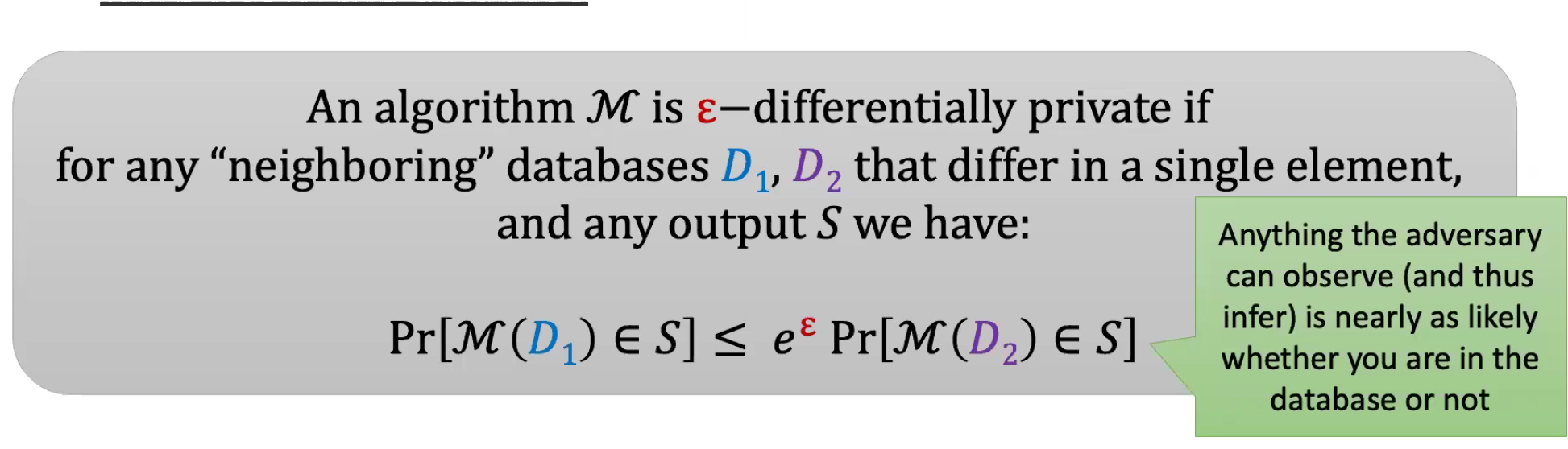
Simple Example: Private Sum Computation
For surveys, add noise to approximate the true sum without reconstructing individual responses.
- Sensitivity: $\delta f = \max_{D_1, D_2} |f(D_1) - f(D_2)|$, where $D_1, D_2$ are neighboring datasets.
- Release $y \sim \text{Laplace}(f(D), \delta f / \epsilon)$, where Laplace noise has quicker tail decay than Gaussian.
Properties
- Post-Processing: If $M$ is $\epsilon$-DP, any function of $M$’s output is also $\epsilon$-DP.
- Composition: If $M_1$ is $\epsilon_1$-DP and $M_2$ is $\epsilon_2$-DP, their composition is $(\epsilon_1 + \epsilon_2)$-DP; privacy degrades but scales linearly.
DP for Machine Learning
- Use Differentially Private Stochastic Gradient Descent (DP-SGD): Add noise to gradient sums.
- Clip gradients to bound sensitivity (e.g., max norm $C$), then add Gaussian noise for relaxed $(\epsilon, \delta)$-DP.
- For $n$ steps, composition yields up to $n\epsilon$-DP, improvable to $O(\sqrt{n} \epsilon)$ with advanced theorems.
- Practical challenges: High noise often degrades performance for full training.

Web-Scale Pretraining and Privacy for Free

Effective Strategy
Pretrain on public data, then fine-tune with DP on private data; leverages transfer learning for noise robustness.
Granularity Considerations
Define privacy units (e.g., word, sentence, document, or group chat) to balance utility and protection.
Alternatives to Private Finetuning
Use zero/few-shot in-context learning for privacy; effective if tasks align with pretraining, but limited for divergent domains.

Membership Inference

Overview
Membership Inference (MI) attacks aim to determine if a specific data point was included in a model’s training set. This can be formalized as a security game: A challenger trains a model on either dataset $D$ or $D \cup \{x\}$, and the adversary guesses which was used. MI exploits differences in model behavior on seen versus unseen data, often due to overfitting.
Relationship with Differential Privacy
- There is a formal connection between MI and Differential Privacy (DP), a framework that bounds information leakage about individuals in a dataset.
- If an algorithm is $\epsilon$-DP, MI success is bounded (adversary advantage is at most $e^\epsilon - 1$). Conversely, if MI is impossible (adversary advantage near zero), the algorithm provides DP-like guarantees.
- MI can empirically upper-bound data leakage or test DP compliance.
Implications
- MI itself leaks minimal data (e.g., binary membership), but worst-case scenarios include revealing sensitive attributes like disease status.
- It serves as a building block for broader attacks, such as data extraction.
- Applications include proving data provenance for copyright litigation, though this may encourage adversarial practices.

Methods for Membership Inference

Basic Approaches
- Prompt the model with a partial sample and check if it completes the rest accurately; success indicates strong evidence of memorization, though not exhaustive.
- Compare loss values: Training data typically has lower loss than held-out data. Statistical tests can detect this, but distributions overlap, complicating thresholds.
- High loss on a sample can confidently prove non-membership.
- Evaluation focuses on False Positive (FP) rate or Area Under the ROC Curve (AUC-ROC) rather than overall accuracy, as conservative decisions are prioritized.
LiRA Attack (Carlini et al., 2022)
- Improves on basic loss tests by accounting for varying sample difficulty.
- Low loss on easy samples (e.g., clear cat image) suggests non-membership; low loss on hard samples (e.g., noisy truck image) is suspicious.
- Uses a likelihood ratio: $\frac{P(\text{loss} \mid x \in \text{training})}{P(\text{loss} \mid x \notin \text{training})}$.
- Approximates distributions via shadow models (surrogate models trained on subsets) modeled as Gaussians for membership tests.
- Achieves high precision on a subset of samples but with elevated FP rates overall.

Applying LiRA to Large Language Models (LLMs)

Adapting Loss Metrics
- For token sequences, use cross-entropy loss, modeling distributions as univariate Gaussians.
- Enhanced version treats each token as a dimension in a multivariate Gaussian, assuming independence or computing covariance for better accuracy (computationally intensive).
Challenges and Alternatives
- Training shadow models per sample is expensive, requiring full LLM retraining.
- Approximation: Train only on held-out data and check if the sample is an outlier.
- Without retraining: Compare losses from alternative LMs; high loss on one but low on the target suggests membership.
  - Use simple proxies like gzip compression size to approximate out-distribution loss.
  - Perturb samples (e.g., change capitalization) and observe loss sensitivity.
- These ad-hoc methods are unreliable and perform poorly in practice.
Evaluation Challenges
- Ground truth is hard to obtain; proxies include post-cutoff books (e.g., after 2021 for older models) as non-members and classics (e.g., Charles Dickens) as members.
- Distribution shifts (e.g., pre-2022 vs. post-2022 data) bias results; simple temporal classifiers outperform many MI attacks.
- Published evaluations are often flawed without baseline adjustments.
- Reliable tests require scratch-trained models like the Pythia suite, where exact training data is known.

Data Provenance Tests

Legal and Practical Considerations
- Aim to prove model training on copyrighted data with low FP rates, which are difficult to achieve reliably.
- Weak claims (e.g., model summarizing a book) are insufficient, as knowledge could stem from summaries.
- All methods remain speculative and “sketchy” without strong statistical backing.
Effective Techniques
- Data Canaries: Select a random string from a large set $C$ (not in existing training data), insert it into your document, and measure target model losses on samples from $C$. Enables statistical tests for membership. Requires proactive insertion, not post-hoc analysis.
- Data Extraction: Prompt the model to regurgitate training data verbatim; providers mitigate this, but jailbreaks can succeed.
  - Basis for lawsuits like The New York Times vs. OpenAI, claiming verbatim reproduction implies training data inclusion.

Niloofar Mireshghallah Guest Lecture

Non-Literal Copying

Beyond Verbatim Reproduction
Copyright lawsuits can extend beyond word-for-word copying; imitation of an artist’s style or semantic elements may constitute infringement, as seen in cases involving generative models producing outputs in the style of protected works.
Utility vs. Copyright Tradeoff
Models must balance utility (e.g., answering factual questions about copyrighted books) with avoiding infringement, ensuring knowledge dissemination without unauthorized reproduction.
Impact of Instruction Tuning
Instruction tuning (fine-tuning LLMs on task-specific instructions to improve alignment) reduces literal copying but increases semantic copying, where concepts or structures are replicated without exact phrasing.
Proposed Fixes
- Reminder Prompts: Inject prompts reminding the model not to copy training data; ineffective in practice, as models can still generate infringing content.
- Memfree Decoding: During generation, check outputs against the training set to prevent memorization-based regurgitation; reduces literal copying but allows non-literal infringement and degrades factual recall.
Extractability vs. Memorization
Extractability refers to the ability to prompt the model to output specific training data, distinct from memorization (internal storage of data). Additional fine-tuning can make previously non-extractable data accessible, highlighting evolving vulnerabilities.

Does Sanitization or Synthetic Data Help?

Sanitization Techniques
- Assess leakage in sanitized datasets, where sensitive information is removed or altered.
- Remove Personally Identifiable Information (PII), such as names or identifiers.
- Obfuscate attributes like location or age by reducing granularity (e.g., “city” instead of exact address).
- Use LLMs to depersonalize text, creating a one-to-one mapping from original to sanitized versions.
Synthetic Data Generation
- Treat original data as a seed to sample synthetic equivalents, aiming to preserve utility while enhancing privacy.
- Vulnerable to reidentification and linking attacks, where anonymized data is matched to individuals using auxiliary information (e.g., known from census or Netflix datasets, where unique combinations enable deanonymization).
- For tabular data, these attacks are straightforward; for text, convert to structured formats and apply semantic matching.
Memorization as a Performance Indicator
In some scenarios, memorization correlates with model performance, suggesting that complete elimination may hinder generalization.

Open Questions and Broader Concerns

Unresolved Research Questions
- Does memorization occur during the Reinforcement Learning (RL) phase of training, such as in Reinforcement Learning from Human Feedback (RLHF)?
- Can models leak memorized data in languages other than the primary training language?
Ethical and Societal Issues
- Consent forms for data usage (e.g., in chatbots) are often unclear, leaving users unaware that interactions are recorded and potentially usable in legal contexts, as highlighted in recent statements by figures like Sam Altman.
- Deepfake research and generative models enable misuse for doxing, stalking, or phishing.
- The field exhibits an “arms race” mentality, prioritizing rapid advancement with limited regard for regular end-users’ privacy and security.

Measure Theory Recap

Language Models: Distributions over Strings

Definition of a Language Model

Global and Local Normalization

Globally Normalized Language Model or Energy Model

Locally Normalized Models

Tight Language Models

Defining the Probability Measure of an LNM

Defining an Algebra over \(\bar{\Sigma}^\infty\) (Step 1)

Defining a Pre-measure (Step 2)

Extending Pre-measure into a Measure (Step 3)

Defining a Sequence Model (Step 4)

Interpreting the Constructed Probability Space

Characterizing Tightness

Modeling Foundations

Representation-Based Language Models

Compatibility of Symbol and Context

Representation-Based Locally Normalized Language Model

Estimating a Language Model

Parameter Estimation

Classical Language Models

Finite-State Language Models

Finite-State Automata (FSA)

Weighted Finite-State Automata (WFSA)

Finite-State Language Models (FSLM)

Normalizing Finite-State Language Models

Locally Normalizing a Globally Normalized Finite-State Language Model

Defining a Parametrized Globally Normalized Language Model

Tightness of Finite-State Models

The n-gram Assumption and Subregularity

Representation-Based n-gram Models

Pushdown Language Models

Context-Free Grammars (CFG)

Weighted Context-Free Grammars (WCFG)

Tightness of Context-Free Language Models

Normalizing Weighted Context-Free Grammars (WCFG)

Single-Stack Pushdown Automata

Weighted Pushdown Automata

Pushdown Language Models

Multi-Stack Pushdown Automata

Neural Network Language Models

Recurrent Neural Networks (RNNs)

General Results on Tightness

Elman and Jordan Networks

Variations on RNNs

Parallelizability: The Achilles’ Heel of RNNs

Representational Capacity of Recurrent Neural Networks

RNNs and Weighted Regular Languages

Example: Deterministic PFSA Encoded via Minsky Construction

One Update Step: From \((q_0, a)\) with next symbol \(b\)

One Sampling Step from \((q_0, b)\)

Turing Completeness of RNNs

Computational Power of RNN Variants

Consequences of Turing Completeness

Transformer-based Language Models

Formal Definition of Transformer Network

Attention Mechanism

Transformer Layers and Blocks

Additional Components

Tightness of Transformer-based Language Models

Representational Capacity of Transformer-based Language Models

Equivalence vs. Homomorphism Equivalence

Inability of Transformers to Recognize Simple Languages

Transformers Can Simulate n-gram Models

Additional Notes

Tokenization: definitions and BPE (Byte Pair Encoding)

Challenges with tokenization

Generation: definitions and sampling adapters

What is a sampling adapter? Why do we need one?

Transfer Learning

Early Contextual Embedding Models

CoVe — Contextualized Word Vectors (2017)

ELMo — Deep Contextual Word Representations (2018)

Transformer-based Transfer Learning

BERT (2019) — Bidirectional Encoder Representations from Transformers

RoBERTa — Robustly Optimized BERT Pretraining

ALBERT — A Lite BERT

ELECTRA (2020)

GPT Family — Decoder-only Transformers

GPT-1 (2018)